
Introduction
- Regression
- Linear Regression
- Classification
- Logistic Regression
- SVM
- KNN
- Decision Tree
- Random Forest / Boosting
- Clustering
- K-means
- HDBSCAN
- Dimensionality Reduction
- PCA
- Representation Learning
- RBM
- DBN
1.1 Linear Regression
-
Introduction :
- Models a linear relationship between input features and a continuous target variable using $\hat{y} = w^T x + b$.
- Equivalently, by augmenting the feature vector with a constant term, $\hat{y} = \theta^T \tilde{x}$, where $\tilde{x} = [1, x_1, \dots, x_d]^T$ and $\theta = [b, w_1, \dots, w_d]^T$.
-
Methods
- Objective : minimize the Mean Squared Error, $MSE = \frac{1}{N}\sum (y_{true} - y_{pred})^2$.
- Closed form (Normal Equation) : directly computes optimal weights.
- $w = (X^TX)^{-1}X^Ty$
- Gradient Descent : iterative method; scales to large $n$ and $d$ where the closed form is infeasible.
- $w := w - \alpha \frac{\partial Loss}{\partial w}$, where $\alpha$ is the learning rate.
-
Discussion
-
Probabilistic view : MSE is the MLE under the assumption that residuals are i.i.d. Gaussian. That is, minimizing MSE equals maximizing the Gaussian log-likelihood. (ML02 Section 1)
-
Regularization : adds a penalty term to the loss function to keep weights small, because large weights make predictions sensitive to small input changes and can fit noise in the training data.
- Lasso (L1) : adds $\lambda |w|_1$; applies a constant $\pm\lambda$ pull toward zero, so it can make some weights exactly zero.
- Ridge (L2) : adds $\lambda |w|_2^2$; shrinks weights toward zero.
-
2.1 Logistic Regression
-
Introduction : The name comes from the logistic function $\sigma(z) = \frac{1}{1 + e^{-z}}$, even though Logistic Regression is used for classification, not regression.
- Computes a linear score: $z = w^T x + b$.
- Converts the score into a probability using a sigmoid (logistic) function: $\hat{p} = P(y=1 \mid x) = \sigma(z)$.
-
Methods
-
Objective : minimize Binary Cross Entropy.
$$ BCE = -\frac{1}{N}\sum \left[y_{true}\log(y_{pred}) + (1-y_{true})\log(1-y_{pred})\right] $$
- BCE gets small when the model assigns high probability to the correct class, and gets large when the model is confidently wrong.
- If $y_{true}=1$, then $BCE = -\log(y_{pred})$.
- If $y_{true}=0$, then $BCE = -\log(1-y_{pred})$.
- BCE gets small when the model assigns high probability to the correct class, and gets large when the model is confidently wrong.
-
Gradient Descent : update the parameters iteratively to reduce the BCE loss.
- $w := w - \alpha \frac{\partial Loss}{\partial w}$ and $b := b - \alpha \frac{\partial Loss}{\partial b}$, where $\alpha$ is the learning rate.
-
Decision boundary : using threshold $0.5$, predict class $1$ if $\hat{p} \geq 0.5$, otherwise class $0$. Since $\sigma(0)=0.5$, the decision boundary is $w^T x + b = 0$.
-
-
Discussion
-
Log-odds view : Logistic Regression models the log-odds as a linear function of the input.
- Odds compare the probability of class $1$ against class $0$: $\frac{p}{1-p}$.
- ex) If $p=0.8$, then odds $= \frac{0.8}{0.2}=4$, so class $1$ is 4 times more likely than class $0$.
$$ \log\frac{p}{1-p} = w^T x + b $$
-
2.2 Support Vector Machine (SVM)
-
Introduction : finds a decision boundary that separates classes with the largest possible margin.
- The margin is the distance between the decision boundary and the closest training points.
- Support vectors are the closest training points that determine the margin.
-
Methods
-
Objective : maximize the margin; soft-margin SVM adds a penalty for margin violations.
- Hard-margin part: margin width is $\frac{2}{\lVert w \rVert}$; maximizing it is equivalent to minimizing $\lVert w \rVert$, commonly written as $\frac{1}{2}\lVert w \rVert^2$.
- Decision boundary: for linear SVM, the boundary is a line/hyperplane $w^T x + b = 0$.
- Margin boundaries: $w^T x + b = 1$ and $w^T x + b = -1$.
- Soft-margin part: add hinge-loss penalty $C \sum_i \max(0, 1 - y_i(w^T x_i + b))$ for points that are misclassified or inside the margin.
- Gives zero penalty to correctly classified points outside the margin, and penalizes points that are inside the margin or misclassified.
$$ \min_{w,b} \frac{1}{2}\lVert w \rVert^2 + C \sum_i \max(0, 1 - y_i(w^T x_i + b)) $$
- Hard-margin part: margin width is $\frac{2}{\lVert w \rVert}$; maximizing it is equivalent to minimizing $\lVert w \rVert$, commonly written as $\frac{1}{2}\lVert w \rVert^2$.
-
Optimization : solve the convex objective to find the optimal $w$ and $b$; classic SVMs use quadratic programming, while large-scale linear SVMs can use SGD.
-
-
Discussion
-
Hard margin vs Soft margin : hard-margin SVM assumes the data is perfectly separable, while soft-margin SVM allows some margin violations using the penalty parameter $C$.
-
Effect of $C$ : large $C$ penalizes violations strongly, so the model tries to classify training data more strictly. Small $C$ allows more violations, which can give a wider margin and better generalization.
-

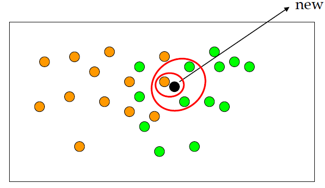
2.3 K-Nearest Neighbors
-
Introduction : predicts a query point by looking at the $k$ most similar training points, based on a distance metric.
-
Methods
- Training : no explicit training; store the training data.
- Evaluation : compute distances from the query point to training points and select the $k$ nearest neighbors.
- Regression : return the mean value of the $k$ nearest neighbors.
- Classification : return the majority class among the $k$ nearest neighbors.
-
Discussion
- k : small $k$ can overfit, while large $k$ can underfit. Use an odd number for binary classification to reduce ties.
- Distance metric : common choices include L1/Manhattan distance and L2/Euclidean distance.
- L1 / Manhattan : sums absolute differences across features.
- L2 / Euclidean : straight-line distance between two points.
2.4 Decision Tree
-
Introduction : a tree-shaped model that predicts by recursively splitting the feature space with simple if-else decision rules.
-
Methods
- Training : greedily build the tree by choosing feature/threshold splits that reduce impurity at each node.
- The model tries candidate thresholds for each feature and chooses the split with the largest impurity reduction.
- Impurity measures how mixed the labels are in a node; a pure node mostly contains one class.
- Impurity reduction: $\Delta I = I(parent) - \frac{N_L}{N}I(left) - \frac{N_R}{N}I(right)$.
- Gini impurity measures how mixed the classes are inside a node; $Gini=0$ means the node is perfectly pure.
- Classification: commonly use Gini impurity $Gini = 1 - \sum_k p_k^2$ or entropy $H = -\sum_k p_k \log p_k$.
- Regression: commonly use MSE reduction.
- The model tries candidate thresholds for each feature and chooses the split with the largest impurity reduction.
- Prediction : follow the decision rules from root to leaf.
- Classification: return the majority class in the leaf.
- Regression: return the mean target value in the leaf.
- Training : greedily build the tree by choosing feature/threshold splits that reduce impurity at each node.
-
Discussion
- Easy to interpret, but can overfit if the tree grows too deep.
- Common controls include
max_depth,min_samples_split, and pruning.
2.5 Random Forest / Boosting
-
Introduction : ensemble tree methods combine multiple decision trees to improve generalization.
-
Methods
- Random Forest (Bagging) : trains many trees independently on bootstrapped samples and averages/votes their predictions.
- Bootstrap Aggregating (Bagging): sample data with replacement, train multiple models, then aggregate their predictions.
- Bagging trains models independently in parallel, then aggregates predictions.
- Reduces variance compared to a single decision tree.
- Boosting : trains trees sequentially, where each new tree focuses on errors made by previous trees.
- Boosting trains models sequentially, where each model tries to correct previous errors.
- Reduces bias by gradually improving weak learners.
- Random Forest (Bagging) : trains many trees independently on bootstrapped samples and averages/votes their predictions.
-
Discussion
- Random Forest is usually more robust and easier to tune.
- Boosting often gives strong accuracy, but is more sensitive to hyperparameters such as number of trees, tree depth, and learning rate.
3.1 K-means
-
Introduction : an unsupervised learning algorithm that partitions data into $k$ clusters by assigning each point to the nearest cluster center.
-
Methods : Repeat assignment and update steps until centroids stop changing or a maximum number of iterations is reached.
- Initialize : choose $k$ initial centroids.
- Assignment step : assign each point to the nearest centroid.
- Update step : recompute each centroid as the mean of the points assigned to it.
- $\mu_k = \frac{1}{\lvert C_k \rvert}\sum_{x_i \in C_k}x_i$
-
Discussion
- Sensitive to the initial centroids, so K-means is often run multiple times with different initializations.
- Sensitive to feature scale, so standardization is often important.
- Works best when clusters are roughly spherical and similarly sized.

3.2 HDBSCAN (Hierarchical DBSCAN, 2013)
-
Introduction : HDBSCAN extends DBSCAN by converting it into a hierarchical clustering algorithm, and then using a technique to extract a flat clustering based in the stability of clusters.
-
Methods :
-
Transform the space according to the density/sparsity.
-
The single-linkage algorithm at the core of hierarchical clustering is extremely sensitive to noise: a single mis-placed noise point can chain two clusters into one. A more robust distance is therefore needed.
-
Mutual Reachability Distance : the MRD between
aandbis the maximum of { distance(a, k-nearest neighbor of a), distance(b, knn of b), distance(a, b) }. In dense regions this falls back to the direct distanced(a,b); in sparse regions it uses each point’s distance to its k-th neighbor instead, making the metric robust to noise. [reference]$$ MRD = max[core_k(a), core_k(b), d(a,b)] $$
-
-
Build the minimum spanning tree of the distance-weighted graph : Treat each data point as a node and connect them with weighted edges whose weight is the MR distance between the two endpoints. The resulting graph is the same regardless of where the construction starts (fig1).
-
Construct a cluster hierarchy of connected components : Walk the edges from the longest MR distance down, lowering a threshold and cutting connections as the threshold decreases.
-
Condense the cluster hierarchy based on minimum cluster size : Prune the hierarchy where a branch would contain fewer points than the specified minimum cluster size.
-
Extract the stable clusters from the condensed tree : we want the choose clusters that persist and have a longer lifetime;
-
4.1 PCA : Principal Component Analysis
-
Introduction : PCA is an unsupervised linear dimensionality reduction method.
- Principal Components : new orthogonal axes that capture the largest variance in the data.
- Projects high-dimensional data onto the top $k$ principal components.
-
Methods
- Standardize : center/scale features before PCA when they have different units or ranges.
- Find principal components : find orthogonal directions that capture the largest variance.
- Principal components are ordered by explained variance.
- Project : map the original data onto the top $k$ principal components.
-
Discussion
- Covariance matrix : summarizes how features vary together; PCA uses it to find directions where the data varies the most.
- Eigen-decomposition : commonly used to compute PCA from the covariance matrix.
- Eigenvectors become principal components.
- Eigenvalues represent explained variance.
- Eigenface : PCA applied to face images; early components capture broad variations such as lighting, pose, and face structure, while later components capture smaller details or noise.

5.1 RBM : Restricted Boltzmann Machine (RBM)
-
Introduction : RBMs are two layered NN with generative capabilities, that have the ability to learn a prob dist over its input. RBMs can be used for dimensionality reduction, classification, regression, and so on.
-
Architecture : Two layers — one input layer and one hidden layer. Unlike a Boltzmann Machine where units in the same layer are connected, in an RBM there are no intra-layer connections (it is restricted in this sense).
-
Training : Trained with Gibbs Sampling — a stochastic algorithm that draws a sequence of samples from the joint distribution of two or more random variables (Unsupervised Learning).
-
The training intuition: feed the input forward, run the activations backward to reconstruct it, and minimize the difference between the reconstruction and the input — much like an autoencoder.
-
forward : $ y_{out} = \sigma (wx + b)$
-
backward (reconstruct the input) : $ y_{recon} = y_{out} x + b$
-
KL Divergence can be considered as the reconstruction error: $ KL(x|y_{recon}) $
-
Reduce KLD in iterative manner : common training algorithms for RBMs approximate the log-likelihood gradient given some data and perform gradient ascest on these approximations.(Gibbs Sampling)
-
5.2 DBN : Deep Belief Network
-
Architecture : Multiple RBMs can also be stacked and can be fine tuned through the process of gradient descent and backpropagation.
-
Train : Once the first RBM is trained, its parameters are frozen and a second RBM is trained using the hidden units of the first as input. The full DBN stack can then be fine-tuned with gradient descent and backpropagation.
-
DBNs drew attention not so much because they modeled the joint probability well, but because using a DBN to pretrain another DNN mitigated overfitting and improved downstream performance.
-
However, with enough data, random initialization is known to outperform DBN-based weight initialization, so DBNs are rarely used in practice today.