
Introduction
-
Tasks:
- Action Classification : The task classfying an action in video sequences according to its spatio-temporal content.
-
Benchmark Set
- UCF-101 : is an action recognition data set of realistic action videos, collected from YouTube, having 101 action categories.
- HMDB-51
- Kinetics : has 400 human action classes with more than 400 examples for each class, each from a unique YouTube video.
-
Methods
-
CNN + RNNs
-
3D Convolutional Networks
- ResNeXt-101 : 6GFLOPs for 112x112x16
-
Two Stream Network (RGB + Optical Flow)
-
Two Stream 3D ConvNets
-
Feature Engineering with pre-extracted frame-level featue using CNN
-
Skeleton Based Recognition using GCN
- ST-GCN : 16 GFLOPs for one action sample
-
1. LRCN : Long-term Recurrent Convolutional Networks (2014)
-
Introduction : previous models assume a fixed visual representation or perform simple temporal averaging for sequential processing (such as action recog, image captioning, or etc).
-
Method : Long-term Recurrent Convolutional Networks that can learn compositional representations in space and time.
2. C3D (2014)
-
Introduction : 3D Convolutional Network for learning spatiotemporal feature from a large scale video dataset
-
Method : 3D ConvNets are just like standard convolutional networks, but with spatio-temporal filters (3x3x3)
3. Two Stream Network (2014)
-
Introduction : investigate architectures to capture the complementary information on appearance from still frames and motion between frames (optical flow).
-
Method : averaging the predictions from a single RGB frame and a stack of 10 externally computed optical flow frames, after passing them through two replicas of an ImageNet pre-trained ConvNet.
4. I3D (2017)
-
Introduction : A number of successful image classification architectures have been developed over the years through painstaking trial and error. Instead of repeating the process for spatio-temporal models, authors propose to simply convert successful image(2D) classification models into 3D ConvNets.
-
Method : Two-Stream Infalted 3D ConvNet (I3D) that is based on 2D ConvNet inflation
-
Inflating 2D into 3D : filters and pooling kernels of 2D ConvNets for image classification are just expanded into 3D.
-
Two 3D Streams : with one I3D network trained on RGB inputs and another on optical flow inputs. Authors trained two networks separately and averaged their predictions at test time.
-
5. ActionVLAD (2017)
-
Introduction : 3D CNN or two stream architectures disregard the long-term temporal structure of video. For example, a basketball shoot, can be confused with other actions such as running, dribbling, jumping, throwing, with only few consecutive frames. So we need a global descriptor for the entire video.
-
Methods:
-
sample frames from the entire video and get top-conv features using a pretrained CNN from RGB and flow each.
-
ActionVLAD : is a learnable spatio temporal aggregation layers. While max or average pooling are good for similar features, actionVLAD aggregates their residuals from nearest cluster centers.
$$ V = \sum_{t=1}^{T} \sum_{i=1}^{N} {\frac{e^{-\alpha || x_{it}-c_k||^2}}{ \sum_{k’} {e^{-\alpha || x_{it} - c_{k’}||^2}}}} (x_{it}[j] - c_k[j]) $$
-
combine VLADs from each stream (get video-level fixed length vector) and pass it through a classifier that outputs the final classification scores.
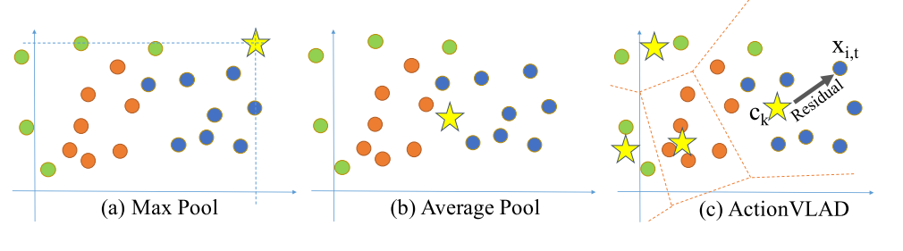
Different pooling strategies for a collection of diverse features. Points correspond to features from a video and colors correspond to different sub-actions in the video. -
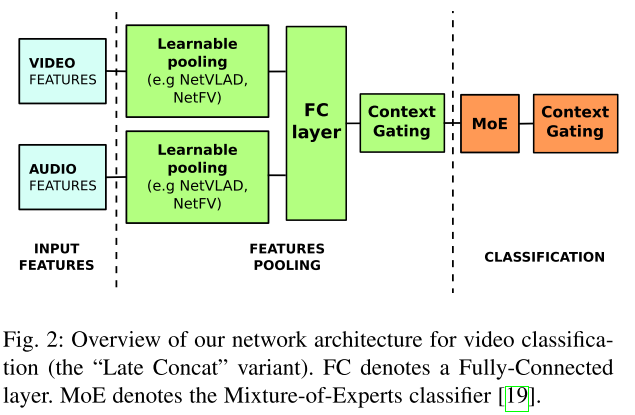
6. LOUPE : 1st place at 2017 Youtube-8M (2017)
-
Introduction : Current method for video analysis often extract frame-level features using pre-trained CNNs. Such features are then aggregated over time e.g., by simple temporal averaging or more sophisticated recurrent neural networks such as LSTM or GRU. This work first explore clustering-based aggregation layers.
-
Method :
-
CNN Feature Extraction: The input features (frame-level) are extracted from video and audio signals.
-
Create Local feature: The pooling module (e.g. netVLAD) aggregates the extracted features into a single compact (e.g. 1024 dim) representation for the entire video.
-
Feature Enhancing: The aggregated representation is then enhanced by the Context Gating Layer.
-
Classification: Classification module takes the resulting representation as input and output scores for a pre-defined set of labels.
-
7. 3D ResNext (2017)
-
Introduction : Conventional research has only explored relatively shallow 3D architectures. Authors examine the architectures of various 3D CNNs from relatively shallow to very deep ones on current video datasets.
-
Method : training 3D CNNs such as ResNet, ResNext, DenseNet on UCF101, HMDB-51 and so on.
8. SlowFast Networks (2018)
-
Introduction : The recognition of the categorical semantics (colors, textures, lighting etc.) can be refreshed relatively slowly. On the other hand, the motion being performed can evolve much faster. So authors present a two-pathway SlowFast model for video recognition
-
Method : simply can be described as a single stream architecture that operates at two different framerates.
-
Slow pathway : can be any spatiotemporal conv model. key concept is a large temporal stride τ (typically 16) on input frames, i.e., it processes only one out of τ frames.
-
Fast pathway : another conv model which have a small temporal stride
-
Lateral Connections : The information of the two pathways is fused by lateral connections which have been used to fuse optical flow based, two-stream networks.
-
9. ST GCN (2018)
-
Introduction : propose a novel model of dynamic skeletons called ST-GCN
-
Methods:
-
Pose Estimation : construct a spatiotemporal graph with the joints as graph nodes and natural connectivities in both human structures and times as graph edges.
-
Skeleton Graph Construntion : The node set $V$ has all the joints in a sequence including estimated coordinates and estimation confidence. The edge set $E$ is composed of two subset, that depicts the intra skeleton connetcion and inter-frame edges.
-
Spatial GCN : The feature map $f^t_{in} : V_t \rightarrow R^c $ has a vector on each node of the graph.
-
on image, convolution opertion can be written as below with sampling function $p$ and weight function $w$.
$$ f_{out}(\mathbb{x}) = \sum_h \sum_w f_{in} (p(\mathbb{x},h,w)) \cdot w(h,w) $$
-
sampling function : On image, neigboring pixels are defined by x as center using kernel size. On graph, neighbor nodes are defined by the minimum length of path from x.
-
weight function : is similart to the kernel of 2d convolution. But we have a mapper
$$ f_{out}(v_{ti}) = \sum_{v_{tj} \in B(v_{ti})} \frac{1}{Z_{ti}(v_{tj})} f_{in}(v_{tj}) \cdot \mathbb{w}(l_{ti}(v_{tj})) $$
-
spatiotemporal modeling : Until now, we formulated spatial GCN, this can be expanded in temporal dimension simply. By extending the concept of neighborhood to also include temporally connected joints
-
-
Partition strategies : design a partitioning strategy to implement the label map $l$.
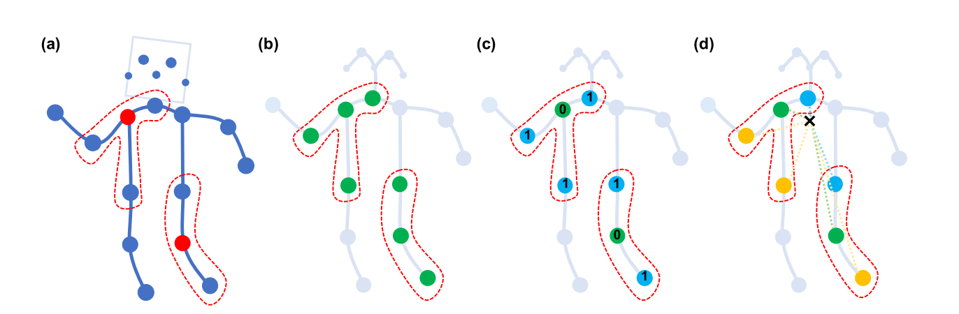
(d) spatial configuration partitioning. The nodes are labeled according to their distances to the skeleton gravity center (black cross), root(green), near(blue), longer(yellow)
-
-
Limitations : cannot model the correlation between the joints that located further away than the maximum distance D. (left hand and right foot) : resolved by Actional Structural GCN
10. Shift GCN (2020)
-
Introduction : propose a novel shift graph convolutional network to overcome conventional shortcomings
-
Computational complexity of GCN based methods are pretty heavy.
-
The receptive fields of both spatial graph and temporal graph are inflexible
-
11. ViViT : A Video Vision Transformer (2021, Goog Res)
-
Introduction : We propose a pure-transformer architecture for video classification, inspired by the recent success of such models for images like ViT.
-
Methods :
-
Embedding video clips : two simple methods for mapping a video to a sequence of tokens $\hat{z}$ (Uniform, Tubelet) and then add the positional embedding and reshape into $z$, the input to the transformer
$$ \mathbf{V} \in \mathbb{R}^{T\times H\times W \times C} \mapsto \hat{z} \in \mathbb{R}^{n_t \times n_h \times n_w \times n_d} \rightarrow z \in \mathbb{R}^{N \times d} $$
-
Uniform frame sampling (Figure2) : simply sample $n_t$ frames, and embed each 2D frame independently following ViT (Conv2D + Concat)
-
Tubelet Embedding (Figure3) : extension of ViT’s embedding to 3D and corresponds to a 3D convolution.
-
-
Transformer Models for VIdeo
-
Model 1) Spatio-temporal attention : simply forwards all spatio-temporal tokens extracted from the video
-
As it models all pairwise interactions, Multi-Headed Self Attention has quadratic complexity with respect to the number of tokens.
-
motivates the development of more efficient architectures
-
-
Model 2) Factorised encoder : consists of two separate transformer encoders
-
spatial encoder : only models interactions between tokens extracted from the same temporal index.
-
temporal encoder: consisting ofLttransformer layers to model in-teractions between tokens from different temporal indices.
-
-
-
-
Results
-
Input Encoding : tubelet embedding initialised using the “central frame” method (Eq. 9) performs well, outperforming the others (Table1)
-
Model Variants : The unfactorised model (Model 1) performs the best on Kinetics 400. However, it can also overfit on smaller datasets such as Epic Kitchens, where we find our “Factorised Encoder” (Model 2) to perform the best
-
12. TimeSformer : Is Space-Time Attention All You Need for Video Understanding (2021)
-
Introduction : We present a convolution-free approach to video classification
-
Methods : TimeSformer (Time-Space Transformer)
-
Preprocessing
-
Input Clip : TimeSformer takes input clip $X \in \mathbb{R}^{H \times W \times 3 \times F}$
-
Decomposition into patches ; each frame is decomposed into $N$ non-overlapping patches of $\mathbf{x_{(p,t)}} \in \mathbb{R}^{3P^2}$
-
Linear embedding : embedding vector $\mathbb{z}{(p,t)} \in \mathbb{R}^D$ by means of a learnable matrix $E \in \mathbb{R}^{D \times 3P^2}$ with trainable positional embedding $e^{pos}{(p,t)} \in \mathbb{R}^D$ : $\mathbf{z}{(p,t)} = E\mathbf{x}{(p,t)} + e^{pos}_{(p,t)}$
-
Classification Embedding : The final clip embedding is obtained from the final block for the classification token, On top of this representation we append a 1-hidden-layer MLP, which is used to predict the final video classes.
- output을 다시 aggregation 해서
-
-
Modelling
-
Query Key Value computation : At each block $l$, a query/key/value vector is computed for each patch from the representation $z^{(l−1)}_{(p,t)}$encoded by the preceding block
-
Self-attention computation : via dot-product of query and key vector
-
Encoding : The encoding is obtained by computing the weighted sum of value vectors using self-attention coefficients from each attention head
-
-
Space-Time Self Attention Models : temporal attention and spatial attention are separately applied one after the other
- we first compute temporal attention by comparing each patch(p,t) with all the patches at the same spatial location in the other frames
-
-
Conclusion : conceptually simple, achieves state of the art results on major action recognition tasks, has low training and inference cost, adn can be applied to clips of over one minute, thus enabling long-term video modeling.
class PatchEmbed(nn.Module):
    self.patch_embed = nn.Conv2d(in_chans, embed_dim, kernel_size=patch_size, stride=patch_size)
    self.cls_token = nn.Parameter(torch.zeros(1, 1, embed_dim))
    self.pos_embed = nn.Parameter(torch.zeros(1, num_patches+1, embed_dim))
     ...

    def forward_features(self, x):
        x, T, W = self.patch_embed(x)
        cls_tokens = self.cls_token.expand(x.size(0), -1, -1)
        x = torch.cat((cls_tokens, x), dim=1)
        x = x + self.pos_embed
       ...


class Attention(nn.Module):
    self.qkv = nn.Linear(dim, dim * 3)
    self.norm1 = norm_layer(dim)
    ...

    def forward(self, x):
        q, k, v = qkv[0], qkv[1], qkv[2]
        attn = (q @ k.transpose(-2, -1)) * self.scale
        attn = softmax(dim=-1)
        x = (attn @ v).transpose(1, 2).reshape(B, N, C)