
Introduction
-
Tasks:
- Image Retrieval : aims to find similar images to a query image among an image dataset.
-
Tech Trend :
-
Conventional Methods : relying on local descriptor matching (scale invariant features - local image descriptors - reranking with spatial verifications)
-
using FC layers : after several conv layers as global descriptors [A Babenko et al, A Gordo et al.]
-
using global pooling methods : from the activations of conv layers.
-
boost the performance : by combining different global descriptors which are trained individually.
-
1.1 BoF, BoW (Bag of Features, Bag of Visual Words)
-
Introduction : BoW is a simplifying representation used in NLP and information retrieval.
-
Methods : BoF groups local descriptors.
-
Local Feature Extraction : Extract local features from image (SIFT, SURF, small img patches)
-
Clustering : Cluster (k-means) extracted features and find center features (codeword) of each cluster
-
Image representation : Represent each image using histogram of codeword.
-
Learning and Recognition :
-
Generative ways : based on Bayesian => classification by histogram of each class
-
Discriminative ways: using classifier like SVM => put histogram into classifier as a feature vector

Figure 1. Overview of BoW -
-
1.2 VLAD (Aggregating Local Descriptors) (2010)
-
Introduction : propose a simple yet efficient way to aggregating local image descriptors into a vector of limited dimension, which can be viewed as a simplification of the Fisher kernel representation.
-
Fisher Vector : transform a input variable-size set of independent samples into a fixed size vector representation
-
A Gaussian Mixture Model (GMM) is used to model the distribution of features(e.g. SIFT) extracted over the image.
-
The Fisher Vector encodes the gradients of the log-likelihood of the features under the GMM, with respect to the GMM parameters.
-
-
VLAD (Vector of Locally Aggregated Descriptor) : is a feature pooling method, which can be seen as a simplification of the Fisher Kernel. VLAD encodes a set of local feature descriptors extracted from an image using a clustering method such as GMM or K-means.
-
accumulate the differences $x-c_i$ for each visual word $c_i$.
-
subsequently $L_2$ normalized by $v = v / ||v||_2$
-
Can be written using $a_k$ that assigns descriptor $x_i$ to specific cluster centres $c_k$.
$$ v_{i,j} = \sum_{x \in C} x_j-c_{i,j} = \sum_{i=1}^N a_k(x_i)(x_i(j)-c_k(j))$$
-
2.1 NetVLAD (2016)
-
Introduction : develop a cnn architecture that aggregates mid-level conv features into a compact single vector representation using generalized VLAD layer, NetVLAD.
-
Methods : (i) extract top conv featues using pretrained CNN (ii) and pool these features using netVLAD
-
netVLAD : The source of discontinuous in VLAD is hard assignment $a_k(x_i)$ of descriptor $x_i$ to specific cluster centres $c_k$. (If $c_k$ is the closest cluster, $a_k=1$, else, $a_k=0$). Authors replace it to soft assignment (softmax of -distances to each clusters).
$$ a_k(x_i) = softmax( -|x_i - c_k |^2) = \frac{e^{-\alpha | x_i| ^2 + 2\alpha c_k x_i + |c_k |^2}}{\sum_{k’} e^{-\alpha | x_i| ^2 + 2\alpha c_k x_i + |c_{k’} |^2}} = \frac{e^{2\alpha c_k x_i + |c_k |^2}}{\sum_{k’} e^{ 2\alpha c_k x_i + |c_{k’} |^2}} = \frac{e^{w_k^T x_i + b_k}}{\sum_{k’} e^{w_{k’}^T x_i + b_{k’}}}$$
$$V(j,k) = \sum_{i=1}^{N} a_k (x_i)(x_i(j) - c_k(j))$$
3.1 Global Descriptors (~2018)
-
SIFT, SPoC : sum pooling from the feature map which performs well mainly due to the subsequent descriptor whitening.
-
MAC , regional MAC : performs max pooling (MAC) over regions then sum over the regional MAC descriptor at the end.
-
GeM: generalizes max and average pooling with a pooling parameter
-
weighted sum pooling, weighted GeM, multiscale RMAC, etc.
-
The performance of each global descriptor varies by dataset as each descriptor has different properties. For example, SPoC activates larger regions on the image representation while MAC activates more focused regions
3.2 SPoC, Sum Pooling of Convolution (2015)
-
Introduction : investigate possible ways to aggregate local deep features to produce compact global descriptors for image retrieval.
-
Methods :
-
Sum pooling : The construction of the SPoC descriptor starts with the sum pooling of the deep features.
$$ \psi_1(I) = \sum_{y=1}^{H} \sum_{x=1}^{W} f(x,y)$$
-
Centering prior : objects of interest ted to be located close to the geometrical center of an image. So, incorporate such centering prior using coefficients $\alpha(w,h)$ , (Gaussian)
$$ \psi_2(I) = \sum_{y=1}^{H} \sum_{x=1}^{W} \alpha(x,y)f(x,y)$$
-
Post processing : The obtained representation $\psi(I)$ is subsequently l2 normalized, then PCA compression and whitening are performed.
-
3.3 MAC, RMAC, Maximum Activation of Convolution (2015)
-
Introduction : revisit both retrieval stages, namely initial search and reranking
-
Method :
-
Maximum Activation of Convolutions (MAC) : the feature vector constructed by a spatial max-pooling over all feature map $\chi_i$ from last conv.
$$ \mathbb{f_{\Omega}} = [f_{\Omega,1}, f_{\Omega,2}, … ,f_{\Omega,K}]^T, with f_{\Omega,i} = max \chi_i(p)$$
-
regional MAC : divide conv feature map to multiple regions(for WxH dim not C) and apply MAC for each regions and post-process it. (l2 and PCA-whitening)
-
Two images are compared with the cosine similarity of the K-dim vector produced as described above.
-
3.4 GeM, Generalized Mean Pooling (2017)
-
Introduction : propose a novel trainable Generalized Mean Pooling layer that generalizes max and average pooling and show that it boosts retrieval performance
-
Method :
-
ConvNet Backbone : given an input image, the output is a 3D tensor $\chi$ of $W \times H \times K$ dimensions
-
GeM : add a pooling layer that takes $\chi$ as an input and produces a vector $\mathbb{f}$ as an output of the pooling process.
$$ \mathbb{f_{\Omega}} = [f_{\Omega,1}, f_{\Omega,2}, … ,f_{\Omega,K}]^T, f_{\Omega,k} = ( \frac{1}{|\chi_k|} \sum_{x \in \chi_k}x^{p_k})^{\frac{1}{p_k}}$$
-
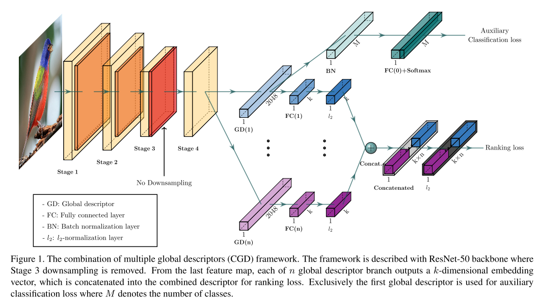
4.1 Combination of Multiple Global Descriptors (2019)
-
Introduction : Ensembling different models and combining multiple global descriptors lead to performance improvement. However, these processes are not only difficult but also inefficient with respect to time and memory. Here, authors propose a novel framework that exploits multiple global descriptors to get an ensemble effect while it can be trained in an end-to-end manner.
-
Method : Proposed framework consists of a CNN backbone and two modules. The first main module learns an image representation, which is a combination of multiple global descriptors. Next, an auxiliary module to fine-tune a CNN with a classification loss.
-
Backbone Network : can use any CNN such as Inception, ShuffleNet, Resnet. authors use ResNet50 as a baseline backbone.
-
Main Module - Multiple Global Descriptors : main module has multiple branches that output each image representation by using different global descriptors (SPoC, MAC, GeM) on the last conv layer. And these discriptions are concatenated after whitening(PCA, FC) and l2 normalization .
-
Auxiliary Module : finetunes the CNN backbone based on the first global descriptor of the main module by using a classification loss (train a CNN backbone with a classification loss and then fine-tune the network with a triplet loss). Additional temperature scaling and label smoothing for performance improvement.
-