0. Introduction

• Tasks :
  • Image Synthesis : The task of creating new images from some form of image description.

---

1. GAN (2014)

• Introduction : A new framework for estimating generative models via an adversarial process

• Method: simultaneously train two models : a generative model $G$ that captures the data distribution, and a discriminative model $D$ that estimates the probability that a sample came from the training data rather than $G$.

$$ \min_{G} \max_{D} V(D,G) = \mathbb{E} _ {x \sim p_{data}(x)} logD(x) + \mathbb{E} _ {z \sim p_z(z)}log(1-D(G(z))) $$

• in terms of Discriminator : $D(x)$ should be 1 and $D(G(z))$ should be 0. So, $D$ is trained to maximize both left and right terms

• in terms of Generator : Left term can be ignored since it’s independent of $G$, and $D(G(z))$ should be 1. So, $G$ is trained to minimize right terms.

• in terms of implementation : We need to make two optimizer. Also G_loss and D_loss should be defined respectively.

---

2. Conditional GAN (2014)

• Introduction : The conditional version of generative adversarial nets, which can be constructed by simply feeding the data, y.

• Method : feeding $y$ into the both the discriminator and generator as additional input layer.

$$ \min_{G} \max_{D} V(D,G) = \mathbb{E} _ {x \sim p_{data}(x)} [logD(x,y)] + \mathbb{E _ {z \sim p_z(z)}[log(1-D(G(z,y),y))].} $$

def generator(x,y):
  input = concat([x,y],1)
  layer1 = relu(FC(input, 128))
  layer2 = tanh(FC(layer1, 784))
  return layer2

def discriminator(x,y):
  input = concat([x,y],1)
  layer1 = lrelu(FC(input, 128))
  layer2 = tanh(FC(layer1, 1))
  return layer2

---

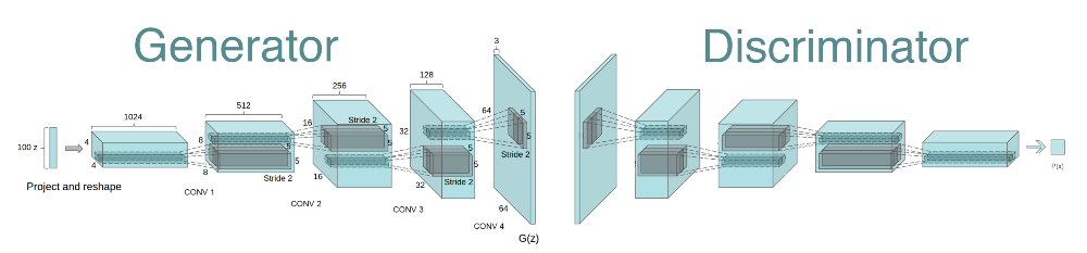
3. DCGAN (2016)

• Introduction : Convolutional GANs that make them stable to train in most settings.

• Method : Following techniques were used for stable Deep Conv GANS.

  1. Replace any pooling layers with strided convolutions (discriminator) and fractional strided convolutions (generator)
  2. Use batchnorm in both the generator and the discriminator
  3. Remove fully connected hidden layers for deeper architectures
  4. Use ReLU for all layers except for the output which uses Tanh
  5. Use LeakyReLU in discriminator for all layers

  

---

4. BEGAN (2017)

• Introduction : A new equilibrium enforcing method paired with a loss derived from the Wasserstein distance for training auto-encoder based GAN.

• Method

  1. use an auto-encoder as a discriminator as was first proposed in EBGAN.
  2. aims to match auto-encoder loss distributions using a loss derived from the Wasserstein distance while typical GANs try to match data distributions directly.
  3. This is done using a typical GAN objective with the addition of an equilibrium term to balance the discriminator and the generator.

$$ L_D = L(x) - k_t L(G(z_d)) $$

$$L_G = L(G(z_G))$$

$$ k_{t+1} = k_t + \lambda (\gamma L(x) - L(G(z_G)))$$

---

5. GIRAFFE (2021)

• Introduction : Deep generative models allow for photorealistic image synthesis at high resolutions content, But this is not enough => creation also needs to be controllable with 3D representation.

  • Our key hypothesis is that incorporating a compositional 3D scene representation into the generative model leads to more controllable image synthesis.

• GIRAFFE : generating scenes in a controllable and photorealistic manner without additional supervision

  • (3.1) model Objects as neural feature fields :

    • NeRF (Neural Radiance Fields) : a function f that maps 3D point and viewing direction to a volume density and RGB color value.
      • Input : single continuous 5D coordinate (spatial location (x, y, z) and viewing direction (θ, φ)),
      • Output : the volume density and view-dependent emitted radiance at that spatial location
      • 2D images from different view => Neural Network => random view image
    • GRAF (Generative Neural Feature Fields) : unsupervised version of NeRF, trained from unposed image collections with additional latent vector.
      • input : spatial location $\gamma(x)$, viewing direction, $\gamma(d)$, shape code $z_s$, appearance code $z_a$
    • GIRAFFE : replace 3D color output with M-dimensional feature from GRAF
      • represent each object using a separate feature field in combination with an affine transformation

• (3.2) Scene Compositions

  • we describe scenes as compositions of N entities where the first N−1 are the objects in the scene and the last represents the background

• (3.3) Scene Rendering

  • 3D Volume Rendering : For given camera extrinsics, maps above evaluations to the pixel’s final feature vector

  • 2D Neural Rendering : maps the feature image to the final synthesized image (2D CNN)

• Result : By representing scenes as compositional generative neural feature fields, we disentangle individual objects from the background as well as their shape and appearance without explicit supervision. Combining this with a neural renderer yields fast and controllable image synthesis.

  • *disentangle : commonly refer to being able to control an attribute of interest, e.g. object shape, size, or pose, without changing other attributes.