
10. Dimensionality Reduction with PCA
- Introduction : Working directly with high-dimensional data comes with some difficulties
- It is hard to analyze,
- interpretation is difficult,
- visualization is nearly impossible,
- and storage of the data vectors can be expensive
- In this chapter, we derive PCA from first principles, drawing on our understanding of
- basis and basis change (Sections 2.6.1 and 2.7.2),
- projections (Section 3.8),
- eigenvalues (Section 4.2),
- Gaussian distributions (Section 6.5),
- and constrained optimization (Section 7.2)
10.1 Problem Setting
-
Objective : is to find projections $\hat{x_n}$ of data points $x_n$ that are as similar to the original data points as possible, but which have a significantly lower intrinsic dimensionality.
-
Dataset : we consider an i.i.d. dataset $X = [x_1 , . . . , x_N], x_n ∈ \mathbb{R}^D,$ with zero mean
-
possesses the data covariance matrix $S$ (6.42)
-
a low-dimensional compressesd representation $z_n$ with the projection matrix $B$
-
$$ S = \frac{1}{N} \sum{x_n}{x_n^⊤} $$
$$ z_n = B^⊤x_n ∈ \mathbb{R}^M $$
$$ B := [b_1,…,b_M] ∈ \mathbb{R}^{D×M} $$
-
Overview
-
We assume that the columns of $B$ are orthonormal (Definition 3.7) so that $b^⊤_i b_j =0 $ if and only if $i \neq j$ and $b^⊤_i b_i =1$.
-
We seek an M-dimensional subspace $U ⊆ \mathbb{R}^D,$ $dim(U)=M < D $ onto which we project the data.
-
We denote the projected data by $\hat{x}_n ∈ U,$ and their coordinates (with respect to the basis vectors $b_1,…,b_M$ of $U$ ) by $z_n. $
-
Our aim is to find projections $ \hat{x_n} ∈ \mathbb{R}^D $ (or equivalently the codes $z_n$ and the basis vectors $b_1, . . . , b_M $) so that they are as similar to the original data $x_n$ and minimize the loss due to compression.
-
10.2 Maximum Variance Perspective
- Introduction :
- We know that the variance is an indicator of the spread of the data, (Section 6.4.1),
- And we can derive PCA as a dimensionality reduction algorithm that maximizes the variance in the low-dimensional representation of the data to retain as much information as possible.
- Centered Data : the variance of the low-dimensional code does not depend on the mean of the data (eq 10.6) Therefore, we assume without loss of generality that the data has mean $0$.
10.2.1 Direction with Maximal Variance
-
(1) Objective : maximize the variance $V_1$ of dataset projected onto single vector $b_1$
-
(2) Variance $V_1$ : expectation of the squared deviation $z_{1n}$
-
$z_{1n}$ is coordinate of the orthogonal projection of $x_n$ onto the one-dim subspace spanned by $b_1$, $z_{1n}$ = $b_1^⊤ x_n$ (section 3.8)
$$ V_1=\frac{1}{N} \sum z_{1n}^2 = \frac{1}{N} \sum b^⊤_1 x_n x_n^⊤ b_1 = b^⊤_1 (\frac{1}{N} \sum x_nx_n^⊤)b_1 = b^⊤_1 S b_1 $$
-
-
(3) Maximize Variance : solve the constrained optimization problem (section 7.2)
- by setting the partial derivatives to 0, gives us the relations
$$ Sb_1 = λ_1 b_1 $$
-
(4) Eigenvalue of Covariance Matrix :
-
By comparing the above relations with the definition of an eigen-decomposition, we see that $b_1$ is an eigenvector of the data covmat $S$ and the Lagrange multiplier $\lambda_1$ plays the role of the corresponding eigenvalue
-
i.e., the variance ($V_1$) of the data projected onto a 1D subspace equals the eigenvalue
-
$$ V_1 = b^⊤_1 S b_1 = λ_1 b^⊤_1 b_1 = λ_1 $$
-
(5) Principal Component :
- Therefore, to maximize the variance, we should find the basis vector associated with the largest eigenvalue (Principal Components), and then project given data onto them.
10.2.2 M-dimensional Subspace with Maximal Variance
-
Extending to $M$dimensional subspace:
- The variance of the data, when projected onto an $M$ dimensional subspace, equals the sum of the eigenvalues that are associated with the corresponding eigenvectors of the data covariance matrix.
$$ V_m = b_m^⊤ S b_m = λ_m b_m^⊤ b_m = λ_m . $$
10.3 Projection Perspective
-
Introduction : Not something new, we will just derive PCA in another view point
-
In the previous section, we derived PCA by maximizing the variance in the projected space to retain as much information as possible.
-
In the following, we will look at the difference vectors between the original data $x_n$ and their projection $\tilde{x}_n$ and minimize this distance so that $x_n$ and $\tilde{x}_n$ are as close as possible.
-
10.3.1 Setting and Objective
- Objective : minimizing the average squared Euclidean distance between $x$ and $\tilde{x}_n$ (projection error)
$$ J_M := \frac{1}{N} \sum | x_n − \tilde{x}_n | ^2 $$
- Solution : To find the coordinates $z_n$ and the OrthoNormalBasis of the principal subspace, we follow a two-step approach
- (1) we optimize the coordinates $z_n$ for a given ONB (10.3.2)
- (2) second, we find the optimal ONB. (10.3.3)
10.3.2 Finding Optimal Coordinates
-
Introduction : Let us start by finding the optimal coordinates $z_{1n} , . . . , z_{Mn}$ of the projections $\tilde{x}_n$ for $n = 1,…,N$ that minimizes the distance between $\tilde{x} − x$.
-
Consequence :
- The optimal linear projection $\tilde{x}_n$ of $x_n$ is an orthogonal projection.
- The coordinates of $\tilde{x}_n$ with respect to the basis $(b_1,…,b_M) $ are the coordinates of the orthogonal projection of $x_n$ onto the principal subspace.
- An orthogonal projection is the best linear mapping given the objective.
-
Summary :
-
So far we have shown that for a given ONB we can find the optimal coordinates by an orthogonal projection onto the principal subspace.
-
In the following, we will determine what the best basis is.
-
10.3.3 Finding the Basis of the Principal Subspace
-
Consequence: after solving the equation from (10.35) to (10.43b), we finally get the consequences below.
- Minimizing the average squared reconstruction (projection) error is equivalent to minimizing the variance of the data when projected onto the subspace we ignore, i.e., the orthogonal complement of the principal subspace
- The basis of the principal subspace comprises the eigenvectors $b_1, … b_M$ that are associated with the largest M eigenvalues of the data covariance matrix.
10.4 Eigenvector Computation and Low-Rank Approximations
-
Introduction
-
In the previous sections, we obtained the basis of the principal subspace as the eigenvectors that are associated with the largest eigenvalues of the data covariance matrix
-
To get the eigenvalues (and the corresponding eigenvectors) of covmat
-
We perform an eigendecomposition (see Section 4.2) : and compute the eigenvalues and eigenvectors of $S$ directly
-
We use a singular value decomposition (see Section 4.5) : Since $S$ is symmetric and factorizes into $XX^T$, the eigenvalues of $S$ are the squared singular values of $X$
-
-
-
Results : The relationship between the eigenvalues of $S$ and the singular values of $X$ provides the connection between the maximum variance view (Section 10.2) and the singular value decomposition.
10.4.1. PCA using Low-Rank Matrix Approximations
-
Eckart-Young theorem: states that $\tilde{X}_M$, is given by truncating the SVD at the top-M singular value.
- Diagonal entries of diagonal matrix $\Sigma_m$ are the $M$ largest singular values of $X$
$$ \tilde{X}_M = U_M \Sigma_M V^T_M $$
10.4.2. Practical Aspects
-
Find eigenvalues and eigenvectors :
-
(1) Roots of the characteristic polynomial (section 4.2) : practically impossible for large matrix.
-
(2) eigendecomposition (or SVD) : we only require a few eigenvectors, so It would be wasteful to compute the full decomposition
-
(3) Iterative methods : If we are interested in only the first few eigenvectors, then iterative processes, which directly optimize these eigenvectors, are computationally efficient
- Power Iteration (Google PageRank) : is very efficient In the extreme case of only needing the first eigenvector.
-
10.5 PCA in High Dimensions
-
Introduction : In the following, we provide a solution to the problem for the case that we have substantially fewer data points than dimensions
- The number of data $N$ is smaller than the dimension of the data $D$.
- The rank of the covmat is $N$, Covmat $S$ has $D-N+1$ eigenvalues that are zero.
- We will turn the $D×D$ covariance matrix into an $N × N$ covariance matrix whose eigenvalues are all positive.
-
Consequences : we can compute the eigenvalues and eigenvectors much more efficiently than for the original $D \times D$ data covmat
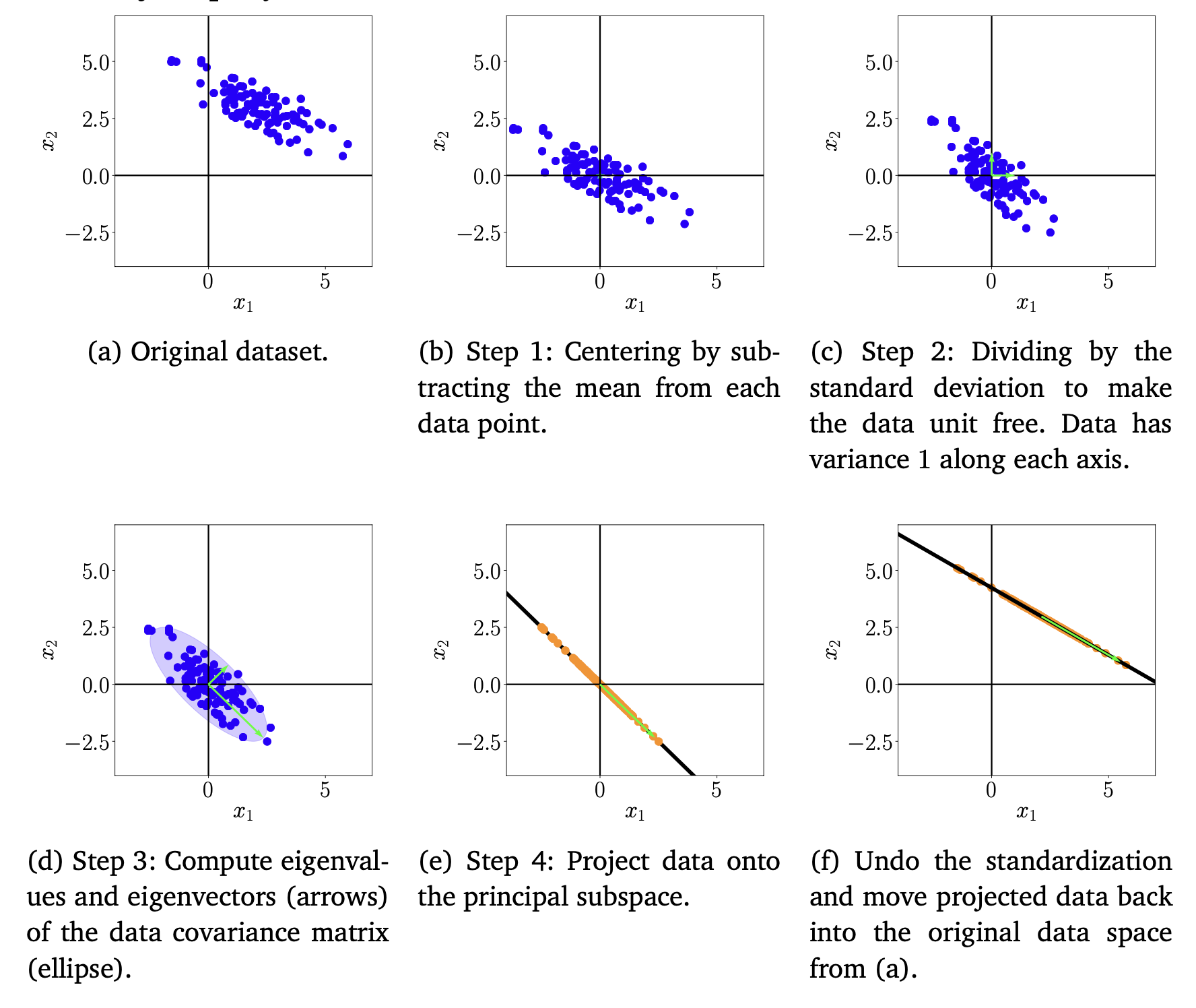
10.6 Key Steps of PCA in Practice
- Introduction : In the following, we will go through the individual steps of PCA using a running example, which is summarized in Figure 10.11
- (1) Mean Subtraction : centering the data by computing the mean and subtracting it from every single data point => dataset has zero-mean
- (2) Standardization : Divide the datapoints by the standard deviation $σ_d$ of the dataset for every dimension.
- (3) Eigendecomposition of the covariance matrix : Compute the data covariance matrix and its eigenvalues and corresponding eigenvectors
- (4) Projection : We can project any data point $x_∗ ∈ R^D$ onto the principal subspace
10.7 Latent Variable Perspective
-
Introduction :
-
In the previous sections, we derived PCA without any notion of a probabilistic model
-
A probabilistic model would offer us more flexibility and useful insights. More specifically, a probabilistic model would
-
Come with a likelihood function, and we can explicitly deal with noisy observations ( which we did not even discuss earlier)
-
View PCA as a generative model, which allows us to simulate new data
-
Have the PCA we derived in earlier sections as a special case
-
-
-
Probabilistic PCA : By introducing a continuous-valued latent variable $z ∈ R^M$ it is possible to phrase PCA as a probabilistic latent-variable model (skip details)
Summary
-
In this chapter, we will discuss principal component analysis, an algorithm for linear dimensionality reduction
-
Section 10.1, Problem Setting
- Our objective is to find projections $\hat{x_n}$ of data points $x_n$ that are as similar to the original data points as possible, but which have a significantly lower intrinsic dimensionality.
-
Section 10.2, Perspective1) Maximum Variance Perspective
-
PCA as a way of dim-reduction that results in the largest variance after projection
-
the variance of projected vectors are same with the eigenvalue of covariance matrix
-
So we can find the best basis vector to project by choose the vector whose eigenvalue is the largest
-
-
-
Section 10.3, Perspective2) Projection Perspective
-
We looked at the difference vectors between the original data $x_n$ and their projection $\tilde{x}_n$ and minimize this distance so that $x_n$ and $\tilde{x}_n$ are as close as possible.
-
Objective : minimizing the average squared Euclidean distance between $x$ and $\tilde{x}_n$ (projection error)
-
An orthogonal projection is the best linear mapping given the objective.
-
-
-
Section 10.4, Eigenvector Computation and Low-Rank Approximations
- Computational efficient ways to find Eigenvector in practical aspect.
-
Section 10.5, PCA in high dimensions
- A solution to the problem for the case that we have substantially fewer data points than dimensions
-
Section 10.6, Key steps of PCA in practice
-
(1) Mean Subtraction
-
(2) Standardization
-
(3) Eigendecomposition of the covariance matrix
-
(4) Projection
-
-
section 10.7, Latent Variable Perspective
- PCA as probabilistic latent-variable model