Mathematics for ML #8 | Introduction Part.II

2022-08-13 3. Mathematics for ML Comments

8. When Models Meet Data

In the first part of the book, we introduced the mathematics that form the foundations of many machine learning methods
The second part of the book introduces four pillars of machine learning:
- Regression (Chapter 9)
- Dimensionality reduction (Chapter 10)
- Density estimation (Chapter 11)
- Classification (Chapter 12)

8.1 Data, Models, and Learning

Three major components of a machine learning system: data, models, and learning.
Good models : should perform well on unseen data.
There are two different senses in which we use the phrase “machine learning algorithm”: training and prediction.

8.1.1 Data as Vectors

We assume that a domain expert already converted data appropriately, i.e., each input $x_n$ is a D-dimensional vector of real numbers, which are called features, attributes, or covariates by following steps:
- Raw Data format : In recent years, machine learning has been applied to many types of data that do not obviously come in the tabular numerical format
- Numerical Representation : Even when we have data in tabular format, there are still choices to be made to obtain a numerical representation.
- Normalization : Even numerical data that could potentially be directly read into a machine learning algorithm should be carefully considered for units, scaling, and constraint

8.1.2 Models as Functions

A predictor is a function that, when given a particular input example (in our case, a vector of features), produces an output

8.1.3 Models as Probability Distributions

Instead of considering a predictor as a single function, we could consider predictors to be probabilistic models,

8.1.4 Learning is Finding Parameters

The goal of learning is to find a model and its corresponding parameters such that the resulting predictor will perform well on unseen data.
we will consider two schools of machine learning in this book, corresponding to whether the predictor is a function or a probabilistic model.
We would like to find good predictors for given training data, with two main strategies :
- based on some measure of quality (sometimes called finding a point estimate),
- using Bayesian inference. (requires probabilistic models)

8.2 Empirical Risk Minimization

In this section, we consider the case of a predictor that is a function

8.2.1 Hypothesis Class of Functions

For given data, we would like to estimate a predictor $f(·,θ):R^D →R$, parametrized by $θ$. We hope to be able to find a good parameter $θ^∗$ such that we fit the data well, that is,

$$ f(x_n,θ^∗) ≈ y_n \text{ for all } n = 1,…,N. $$
- Affine functions (linear functions) are used as predictors for conventional ML methods
- Instead of a linear function, we may wish to consider non-linear functions as predictors.
Given the class of functions, we want to search for a good predictor. We now move on to the second ingredient of empirical risk minimization: how to measure how well the predictor fits the training data.

8.2.2 Loss Function for Training

Equation below is called the empirical risk and depends on three arguments, the predictor $f$ and the data $X, y$.

$$ R_{emp}(f,X,y) = \frac{1}{N} \sum_{n}^{N} l(y_n, \hat{y}_n) $$

Empirical risk minimization : This general strategy for learning is called empirical risk minimization

8.2.3 Regularization to Reduce Overfitting

The aim of training a ML predictor is so that we can perform well on unseen data
Overfitting : the predictor fits too closely to the training data and does not generalize well to new data
Regularization : introduce a penalty term that makes it harder for the optimizer to return an overly flexible predictor
- The simplest regularization strategy is to replace the least-squares problem with the regularized problem by adding a penalty term

$$ \text{min}_θ \frac{1}{N}∥y − Xθ∥^2 \rightarrow \text{min}_θ \frac{1}{N}∥y − Xθ∥^2 + {λ∥θ∥}^2 $$

8.2.4 Cross-Validation to Assess the Generalization Performance

Partitions the data into $K$ chunks, $K-1$ of which form the trainig set, and the last chunk serves as the validation set.
We cycle through all possible partitionings of validation and training sets and compute the average generalization error of the predictor

8.3 Parameter Estimation

In this section, we will see how to use probability distributions to model our uncertainty due to the observation process and our uncertainty in the parameters of our predictors.

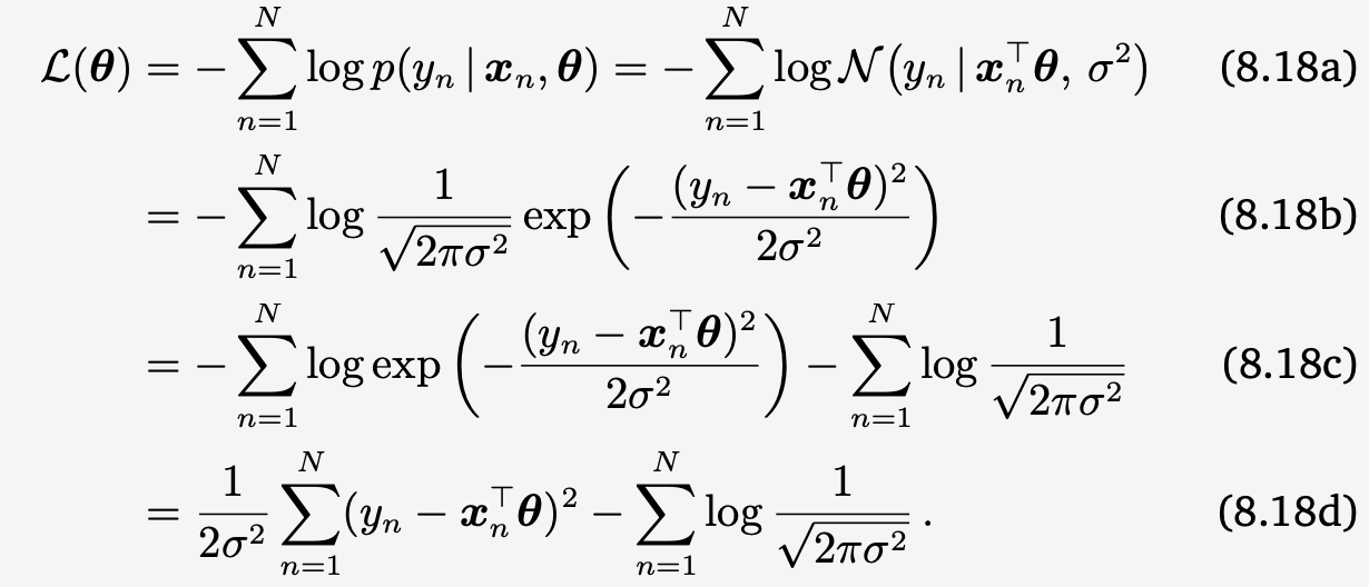
8.3.1 Maximum Likelihood Estimation

The idea behind MLE is to define a function of the params that enables us to find a model that fits the data well.
Negative log-likelihood for data represented by a random variable $x$ and a family of probability densities $p(x|θ)$ is given by :
- The notation $L_x(θ)$ emphasizes the fact that the parameter $θ$ is varying and the data $x$ is fixed.
- To find a good parameter vector $θ$ that explains the data well, minimize the negative log-likelihood $L(θ)$ with respect to $θ$.
$$ L_x(\theta) = −logp(x|θ) $$
Minimizing Neg Log Likelihood $L(θ)$ of Gaussian, corresponds to solving the least-squares problem (below)
- Detail explains : We decided to use Gaussian Distrib to represent given dataset $x_n$, find good param $\theta$ by minimizing Negative Log Likelihood
  - Log : We use log due to the exp term in Gaussian
  - Negative : We use negative because of negative in exp term in Gaussian
- Likelihood and Posterior : details in section 6.3

8.3.2 Maximum A Posteriori Estimaion

If we have prior knowledge about the distribution of the parameters θ, we can multiply an additional term to the likelihood.
Using Bayes’ theorem (6.3) we can compute a posterior distbution $p(θ|x)$, with prior distribution $p(\theta)$, and likelihood $p(x|θ)$

$$ p(θ|x) ∝p(x|θ)p(θ) $$

Instead of estimating the minimum NLL, we now estimate minimum of the negative log-posterior : Maximum a posteriori estimation
Including prior knowledge => regularization, which introduces an additional term that biases the resulting parameters to be close to the origin.

8.3.3 Model Fitting

Overfitting : refers to the situation where the parametrized model class is too rich to model the dataset
Underfitting : we encounter the opposite problem where the model class is not rich enough

8.4 Probabilistic Modeling and Inference

We often build models that describe the generative process that generates the observed data.
- A coin-flip experiment can be described in two steps,
  - (1) we define a parameter μ, which describes the probability of “heads” as the parameter of a Bernoulli distribution
  - (2) we can sample an outcome x ∈ {head, tail} from the Bernoulli distribution $p(x | μ) = Ber(μ)$
In this chapter, we will discuss how probabilistic modeling can be used for this purpose.

8.4.1 Probabilistic Models

Probabilistic models represent the uncertain aspects of an experiment as probability distributions.
In probabilistic modeling, the joint distribution $p(x, θ)$ of the observed variables $x$ and the hidden parameters $θ$ is of central importance: It encapsulates information from the following:
- The prior and the likelihood (product rule, Section 6.3)
- The marginal likelihood p(x), which will play an important role in model selection (Section 8.6), can be computed by taking the joint distribution and integrating out the parameters (sum rule, Section 6.3)
- The posterior, which can be obtained by dividing the joint by the marginal likelihood.
Only the joint distribution has this property. Therefore, a probabilistic model is specified by the joint distribution of all its random variables.

8.4.2 Bayesian Inference

Bayesian Inference
- In Section 8.3.1, we already discussed two ways for estimating model parameters θ using maximum likelihood or maximum a posteriori estimation.
- Once these point estimates $θ^$ are known, we use them to make predictions. More specifically, the predictive distribution will be $p(x | θ^)$, where we use $θ^*$ in the likelihood function.
- Having the full posterior distribution around can be extremely useful and leads to more robust decisions.
  - Bayesian inference is about finding this posterior distribution
  - $p(\theta|X) = \frac{P(X|\theta) p(\theta) }{p(X)}, p(X) = \int{ p(x|\theta) p(\theta) d \theta}$
- The key idea is to exploit Bayes’ theorem to invert the relationship between the parameters $θ$ and the data $X$ (given by the likelihood) to obtain the posterior distribution $p(θ | X )$.
- More specifically, with a distribution p(θ) on the parameters our predictions will be no longer depend on the model param $\theta$, which have been marginalized/integated out.
  - $p(x) = \int p(x | θ)p(θ)dθ$
Parameter Estimation (MLE, MAP) vs Bayesian Inference
- Param estimation : yields a consistent point $\theta^*$ of the parameters
  - the key computational problem to be solved is optimization
- Bayesian Inference : yields a (posterior) distribution
  - the key computational problem to be solved is integration

8.4.3 Latent Variable Models

In practice, it is sometimes useful to have additional latent variables $z$ (besides the model parameters $θ$) as part of the model.
Latent variables may describe the data-generating process, thereby contributing to the interpretability of the model.
The conditional distribution $p(x | θ,z)$ allows us to generate data for any model parameters and latent variables.

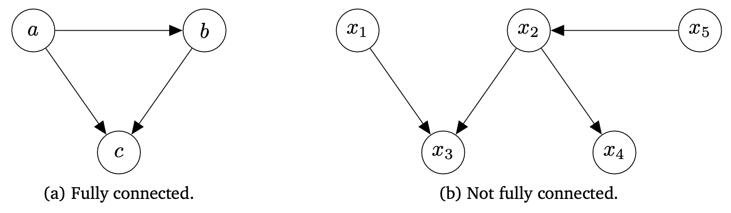
8.5 Directed Graphical Models

In this section, we introduce a graphical language for specifying a probabilistic model, called the directed graphical model
- provides a compact and succinct way to specify probabilistic models,
- allows the reader to visually parse dependencies between random variables
This section relies on the concepts of independence and conditional independence, as described in Section 6.4.5.
Probabilistic graphical models have some convenient properties:
- They are a simple way to visualize the structure of a probabilistic model.
- They can be used to design or motivate new kinds of statistical models.
- Inspection of the graph alone gives us insight into properties, e.g., conditional independence.
- Complex computations for inference and learning in statistical models can be expressed in terms of graphical manipulations.
Ex) The arrow between a and b in Figure 8.9(a) gives the conditional probability $p(b|a) $,
- c depends directly on a and b.
- b depends directly on a.
- a depends neither on b nor on c.

8.6 Model Selection

In machine learning, we often need to make high-level modeling decisions that critically influence the performance of the model
More complex models are more flexible in the sense that they can be used to describe more datasets
- A polynomial of degree 1 (a line) can only be used to describe linear relations between inputs x and observations y.
- A polynomial of degree 2 can additionally describe quadratic relationships between inputs and observations.
However, we also need some mechanisms for assessing how a model generalizes to unseen test data. => Model selection is concerned with exactly this problem.

Summary

In this chapter, We will see how ML algorithms work from a mathematical point of view.
Section 8.1, Data, Model, Learning
- Three main components of ML algorithm : Data, Model, Learning
  - Data as vectors
  - Models as Funtions or Probability Distrib
  - Learning is Finding Parameters
Section 8.2, Empirical Risk Minimization
- ML model as a functional optimization
  - Loss Function : Empirical Risk Minimization (ex. MSE => Least Square Problem)
  - Regularization : additional penalty term in loss function
Section 8.3, Parameter Estimation
- Parameter estimation of data distribution (in terms of ML model training)
  - Likelihood (as loss function)
  - Prior (as regularization term)
Section 8.4 Probabilistic Modeling and Inference
- Bayesian Inference : yields a (posterior) distribution
Section 8.5 Directed Graphical Models
- Directed Graphical Models can be used to specify a probabilistic model.
Section 8.6 Model Selection
- How can we choose the model that works best for unseen data among trained models.