
6. Probability and Distributions
- Probability, loosely speaking, concerns the study of uncertainty
- Probability can be thought of
- as the fraction of times an event occurs,
- as a degree of belief about an event.
- Probability can be thought of
- We then would like to use this probability to measure the chance of something occurring in an experiment
- In ML, we often quantify
- uncertainty in the data,
- uncertainty in the machine learning model, and
- uncertainty in the predictions produced by the model.
- In ML, we often quantify
- Random Variable : Quantifying uncertainty requires the idea of a random variable, which is a function that maps outcomes of random experiments to a set of properties that we are interested in.
- Probability Distribution : Associated with the random variable is a function that measures the probability that a particular outcome (or set of outcomes) will occur
6.1 Construction of a Probability Space
- The theory of probability aims at defining a mathematical structure to describe random outcomes of experiments.
- ex) Coin toss => cannot determine the outcome => by doing a large number of coin tosses => we can observe a regularity in the average outcome.
- Using this mathematical structure of probability, the goal is to perform automated reasoning.
6.1.1 Philosophical Issues
- When constructing automated reasoning systems,
- Boolean logic : does not allow us to express certain forms of plausible reasoning.
- Probability theory : can be considered as a generalization of classic Boolean logic
- Two major interpretations of probability
- Bayesian interpretation : uses probability to specify the degree of uncertainty that the user has about an event, degree of belief
- ex) In Brain MR, a 2cm circle has a 50% chance of being cancer.
- Frequentist interpretation : considers the relative frequencies of events of interest to the total number of events that occurred
- ex) If you toss a coin 100 times, the probability of getting heads is 50%
- Bayesian interpretation : uses probability to specify the degree of uncertainty that the user has about an event, degree of belief
6.1.2 Probability and Random Variables
-
Three distinct ideas that are often confused when discussing probabilities
- Probability space : allows us to quantify the idea of a probability
- Random Variables : transfers the probability to a more convenient (often numerical) space
- Distribution (or law) with a random variable (6.2)
-
Three concepts introduced by Kolmogorov :
- The sample space, Ω : the set of all possible outcomes of the experiment
- For example, two successive coin tosses have a sample space of {HH, TT, HT, TH}
- The event space, A : the space of potential results of the experiment, obtained by considering the collection of subsets of Ω
- The probability, P : We associate(map) a number $P(A)$ that measures the probability or degree of belief that the event will occur.
- The sample space, Ω : the set of all possible outcomes of the experiment
-
Random Variable : a function takes an element of Ω and returns a particular quantity of interest $x$, a value in $T$ (target space), This mapping from Ω to $T$ is called a random variable.
- ex) Tossing two coins and counting the number of heads, a RV $X$ maps to the three possible outcomes $X(hh) = 2, X(ht)=X(th)=1, X(tt)=0$, In this case target space $T = {0,1,2 }$
The name “random variable” is a great source of misunderstanding as it is neither random nor is it a variable. It is a function
6.1.3 Statistics
- Probability theory and Statistics : are often presented together, but they concern different aspects of uncertainty.
- In Probability : we use the rules of probability to derive what happens.
- In Statistics : we observe that something has happened and try to figure out the underlying process that explains the observations
- Machine Learning : close to statistics in its goals to construct a model that represents the process that generated the data
6.2 Discrete and Continuous Probabilities
- Discrete Target space T :
- Random Variable X : takes a particular value x ∈ T,
- Probability Mass Function : the probability that a random variable X takes a particular value x ∈ T , denoted as P (X = x)
- Continuous Target space T :
- Random Variable X : is in an interval, denoted by P(a<X<b)
- Cumulative distribution function : the probability that a random variable X is less than a particular value x, denoted by P (X < x).
- Number of variable
- univariate distribution : distributions of a single random variable
- multivariate distributions : more than one random variable
6.2.1 Discrete Probabilities
- Probability Mass Function : A function that gives the probability that a discrete random variable is exactly equal to some value.
- Random Variable $X$ maps elements in event space to target space.
- ex) Available events {TT, TH, HT, HH} => number of Heads {0,1,2}
- Probability Mass Function $P$ maps elements in target space to probability
- ex) $P(X=0)= \frac{1}{4}, P(X=1)= \frac{2}{4}, P(X=2)= \frac{1}{4} $
- Random Variable $X$ maps elements in event space to target space.
- Joint Probability $p(x,y)$ : is the probability of the intersection of both events, that is $P(X =x_i ∩ Y =y_j) = P(X=x_i, Y=y_j)$
- Marginal Probability $p(x)$ : takes the value $x$ irrespective of the value of random variable $Y$ that is $P(X=x_i)$
- $X∼p(x)$ : denote that the random variable X is distributed according to $p(x)$
- Conditional Probability $p(y|x)$: If we consider only the instances where (X = x), then the fraction of instances for which $Y = y$
6.2.2 Continuous Probabilities
- Probability Density Function: A function $f : R^D → R$ is called a probability density function if :
- $∀x∈R^D :f(x)>0$
- Its integral exists and $ \int_{R^D} f(x)dx = 1 $.
- Probability : $P(a<X<b)=\int_a^b f(x)dx,$
- The probability of a continuous random variable X taking a particular value P (X = x) is zero.
- Cumulative Distribution Function
- CDF of a multivariate real-valued random variable X with states $x ∈ R_D$ is given by $F_X(x) = P(X_1<x_1,…,X_D<x_D)$
- Probability vs Likelihood
6.3 Sum Rule, Product Rule, and Bayes’ Theorem
6.3.1 Sum Rule : the relationship between joint prob and marginal prob.
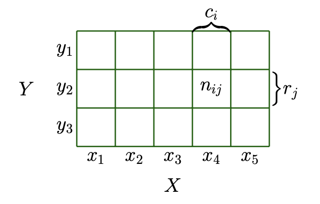
-
(1) Let’s begin with the joint distribution, $p(x,y) = p(X=x_i, Y=y_j) = \frac{n_{ij}}{N}$ of two random variables $x,y$ (figure 6.2)
-
(2) Corresponding marginal distribution $p(x)$ is same with the summation $\frac{c_i}{N} = p(x_i,y_1 ) + p(x_i,y_2) + p(x_i,y_3)$
- $ p(x) = p(X=x_i) = \Sigma_j{p(X=x_i, Y=y_j)} , \ \text{(y is discrete)} $
- $ p(x) = \int_y p(x,y)dy, \ \text{(y is continuous)} $
6.3.2 Product Rule : the relationship between joint prob and cond prob.
- (1) Let’s see the figure6.2 again, conditional distribtion is $p(Y=y_j|X=x_i) = \frac{n_{ij}}{c_i}$
- (2) relates the joint distribution to (1) $p(X=x_i, Y=y_j) = \frac{n_{ij}}{N}$ which is equal to $\frac{n_{ij}}{c_i} \times \frac{c_i}{N}$
$$ p(x, y) = p(y | x)p(x)= p(x | y)p(y) $$
6.3.3 Bayes’ theorem
-
Introduction :
-
In ML and Bayesian statistics, we are often interested in making inferences of unobserved (latent) random variables
-
Bayes’ theorem (6.23) allows us to invert the relationship between x and y given by the likelihood
-
-
Bayes’ theorem : if we have some prior knowledge $p(x)$ and some relationship $p(y|x)$, and observe $y$, we can use Bayes’ theorem to draw some conclusions about $x$.
$$ p(x|y) = \frac{p(y|x)p(x)}{p(y)} $$
-
Posterior, $p(x|y)$ is the quantity of interest in Bayesian statistics
-
Likelihood, $p(y|x)$ : describes how x and y are related, and in the case of discrete probability distributions, it is the probability of the data y
-
Prior, $p(x)$ : encapsulates our subjective prior knowledge of the unobserved (latent) variable x before observing any data.
-
Evidence (marginal likelihood), $p(y)$ : is independent of x, and it ensures that the posterior $p(x|y)$ is normalized.
-
There’s a drug test that is 95% accurate. and assume that 1% of population uses the drug.
Q. If a randomly selected person tests positive for the drug test, what’s the probabiliy that the person is actually a drug user
A. $p(x|y) = \frac{p(y|x)p(x)}{p(y)} = \frac{0.95 \times 0.01}{0.95 \times 0.01 + (1-0.95)*(1-0.01) } \simeq 0.16$
- Let $X$ be the event of an actual drug user and $Y$ the event of a positive result from drug test.
6.4 Summary Statistics and Independence
- We will describe two well known summary statistics : mean and variance
- We will discuss two ways to compare two random variables : independece and inner product
6.4.1 Mean and Covariance (population mean and cov)
-
Expected Value : the expected value of a function $g$ is given by,
- $ E_x[g(x)] = \int_x{g(x)p(x)dx}$ , (For a univariate continuous random variable)
- $E_x[g(x)] = \Sigma_x g(x)p(x)$, (For a discrete random variable)
-
Mean : is an average and is defined as,
-
$E_{x_d} = \int_x x_dp(x_d) dx_d$ ($X$ is a continous random variable)
-
$E_{x_d} = \Sigma_{x_i} x_ip(x_d=x_i)$ ($X$ is a discrete random variable)
-
Details
-
Mean depends on given sample : e.g.) dice roll five times => {1,2,5,2,3} => mean is 2.6 but expectation is 3.5
-
Average : There are many kinds of mean, such as arithmetic, harmonic. Average is same with arithmetic mean.
-
median : is the middel value if we sort the values
-
mode : the most frequently occuring value
-
-
-
Covariance (Univariate): is given by the expected product of their deviations from their respectvive means.
-
Covariance (Multivariate) : The notation of covariance can be generalized to multivariate random variables
-
Covariance Matrix : a square matrix giving the covariance between each pair of elements of a given random vector.
-
References. https://blog.naver.com/sw4r/221025662499
$$ Cov[x,y] = \mathbb{E}[ (x-\mathbb{E}_X(x) )] [(x-\mathbb{E}_Y(y))] = \mathbb{E[(x-\mu_x)(y-\mu_y)]} $$
-
-
Variance : The covariance of a variable with itself $Cov[x,x]$ is called variance and is denoted by $\mathbb{V}_X (x)$
$$ \mathbb{V}_X (x) = Cov_X[x,x] $$
-
Correlation : The normalized version of covariance, the correlation matrix is the cov matrix of standardized random variables, $x/\sigma{(x)}$
$$ corr[x,y] = \frac{Cov[x,y]}{\sqrt{\mathbb{V}(x)\mathbb{V}[y]}} \in [-1,1] $$
6.4.2 Empirical Means and Covariances
-
To compute the statistics for a particular dataset, we would use the observations $x_1, … ,x_N$ and use following
-
Empirical Mean : Empirical mean vector is the arithmetic average of the observations for each variable
- $\hat{x} := \frac{1}{N} \sum_n x_n $
-
Covariance : a DxD matrix
- $\Sigma := \frac{1}{N} \sum_n (x_n -\hat{x})( x_n - \hat{x})^⊤$
-
6.4.3 Three Expressions for the Variance
-
The standard definition of variance (corresponding to the definition) : the expectation of the squared deviation of a randeom variable X from its expected value $\mu$
$$ \mathbb{V}_X(x) := \mathbb{E}_X[(x-\mu)^2] $$
-
Raw score formula : When estimating variance in 6.43, we need to calculate the mean $\mu$ first and we also need to calculate $\hat{\mu}$. We can avoid this two passes by rearranging the terms : so called raw-score formula
$$ \mathbb{V}_X(x) = \mathbb{E}_X[x^2] - \mathbb{E}_X(x)^2 $$
-
Sum of pairwise differences
$$ \frac{1}{N} \sum_{i,j}^N (x_i - x_j)^2 $$
6.4.4 Sums and Transformations of Random Variables
-
Manipulations of Random Variables
-
$\mathbb{E}[x \pm y] = \mathbb{E}(x) \pm \mathbb{E}[y]$
-
$\mathbb{V}[x \pm y] = \mathbb{V}(x) + \mathbb{V}[y] \pm Cov[x,y] \pm Cov[y,x]$
-
-
ex) Consider a random variable $X$ with mean $\mu$ , covmat $\Sigma$, and a affine transformation $y = Ax + b$
-
$\mathbb{E}[y] =\mathbb{E}[Ax+b] = A\mathbb{E}(x) + b = A\mu + b$
-
$\mathbb{V}[y] = \mathbb{V}_X[Ax+b] = \mathbb{V}_X[Ax] =A \mathbb{V}(x)A^⊤ = A\Sigma A^⊤$
-
$Cov[x,y] = \mathbb{E}[x(Ax+b)^⊤] - \mathbb{E}(x)\mathbb{E}[Ax+b]^⊤ = \Sigma A^⊤$
- where $\Sigma = \mathbb{E}[xx^⊤] = \mu \mu^⊤$ is the covariance of $X$
-
6.4.5 Statistical Independence
-
Independence : Two random variables X, Y are statistically independent if and only if $p(x, y) = p(x)p(y) .$
-
$p(y | x) = p(y) $
-
$p(x | y) = p(x) $
-
$ \mathbb{V}_{X,Y} [x + y] = \mathbb{V}_X (x) + \mathbb{V}_Y [y]$
-
$Cov_{X,Y} [x, y] = 0$
- Two RV can have covariance zero but not statistically independent
-
-
Conditional Independence : Two RV X and Y are conditionally independent given $Z$ if and only if:
- $p(x,y|z)=p(x|z)p(y|z) \ \text{for all } z∈Z$
6.4.6 Inner Products of Random Variables
-
Inner product between random variables : $<X,Y> := Cov[x,y]$
-
The length of random variables : standard deviation
- $∥X∥ = \sqrt{Cov[x, x]} = \sqrt{V(x)} = σ(x)$
- The longer the random variable, the more uncertain it is
-
The angle $\theta$ between two random variables : correlation
- $ cos θ = \frac{{X,Y}}{∥X∥∥Y∥} = \frac{Cov[x,y]}{\sqrt{V(x)V[y]}} = corr[x,y]$
-
6.5 Gaussian Distribution
- Gaussian Distribution has many computationally convenient properties, which we will be discussing in the following chapters
- ch9. use Gaussian Distribution to define the likelihood and prior for linear regression
- ch11. mixture of Gaussians for density estimation
- Univariate Gaussian Distribution
- $p(x|\mu, \sigma^2) = \frac{1}{\sqrt{2 \pi \sigma^2}}exp(-\frac{(x-\mu)^2)}{2 \sigma^2})$
- Multivariate Gaussian Distribution : is fully characterized by a mean vector $\mu$ and a cov matrix $\Sigma$
- Standard normal distribution : the special case of the Gaussian with zero mean and identity covariance, that is, $\mu=0$ and $\Sigma=I$
6.5.1 Marginals and Conditionals of Gaussians are Gaussians
- The marginal distribution of $p(x)$ of joint Gaussian distrib $p(x,y)$ is itself Gaussian and computed by applying the sum rule :
- $p(x) = \int{p(x,y)dy} = N(x|\mu_x, \Sigma_{xx})$
- The conditional distribution $p(x|y)$ is also Gaussian and given by
- $p(x|y) = N(\mu_{x|y}, \Sigma_{x|y})$
6.5.2 Product of Gaussian Densities
- The product of two Gaussians $ N(x|a,A), N(x|b,B)$ is a Gaussian distribution scaled by $c ∈ R$, given by $c N(x |\mathbf{c,C} )$ with
- $c = (2π)^{−D/2} |A+B|^{−1/2} exp( \frac{-1}{2}(a−b)^⊤(A+B)^{−1}(a−b))$
- $\mathbf{c} = C(A^{-1}a + B^{-1}b)$
- $\mathbf{C} = (A^{-1} + B^{-1} )^{-1}$
6.5.3 Sums and Linear Transformations
- If $X, Y$ are independent Gaussian random variables (i.e., the joint distribution is given as $p(x, y) = p(x)p(y)$ with $p(x) = N(x | μ_x, Σ_x)$ and $p(y) = N(y | μ_y , Σ_y)$,
- then $x + y$ is also Gaussian distributed and given by $ p(x+y) = N (μ_x +μ_y, Σ_x +Σ_y)$.
6.5.4 Sampling from Multivariate Gaussian Distrib.
-
Sampling from multivariate Gaussian Distrib. $N(0,I)$
-
(1) We need a source of pseudo-random numbers that provide a uniform sample in the interval [0,1]
-
(2) We use a non-linear transformation such as the Box-Muller transform to obtain sample from a univariate Gaussian
-
(3) We collate a vector of these samples to obtain a sample from a multivariate standart normal $N(0,I)$
-
-
Obtain samples from a multivariate normal $N(\mu, \Sigma)$
-
use the properties of a linear transformation of a Gaussian random variable :
-
If $x~N(0,I)$, $y = Ax+\mu$, $AA^T = \Sigma$ is Gaussian distributed with mean $\mu$ and covariance matrix $\Sigma$
-
One convinient choice of $A$ is to use the Cholesky decomposition (section 4.3)
-
-
6.6 Conjugacy and the Exponential Family
-
Bernoulli Distrib.
-
A discrete distrib having two possible outcomes $x ∈ [0, 1]$ in which $x=1$ occurs with probability $p$ and $x=0$ occurs with probability $1-p$
-
$P(x)=p^x(1−p)^{1−x}, x∈ { 0,1 }$
-
$\mathbb{E}(x) = 1 \times p + 0 \times (1-p) = p$
-
$\mathbb{V}(x) = \mathbb{E}[X^2] - (\mathbb{E}[X])^2 = p - p^2 = p (1 - p)$
-
-
ex) when we are interested in modeling the probability of “heads” when flipping a coin
-
References. Bernoulli Distribution, Binomial Distribution
-
-
Binomial Distrib.
-
a generalization of the Bernoulli distribution to a distribution over integers (The number of ways in which y out of N trials can be successful => N combination y)
-
$P(Y=y)= \begin{pmatrix} N \ y \end{pmatrix} p^y(1−p)^{N−y}$
-
$\mathbb{E}(x) = Np$
-
$ \mathbb{V}(x) = Np (1 - p)$
-
-
ex) observing m “heads” in N coin-flip experiments if the probability for observing head in a single experiments is $\mu$
-
-
Beta Distrib.
-
a distribution over a continuous random variable $x ∈ [0, 1]$, which is often used to represent the probability for some binary event
-
$P(x|α,β)= \frac{Γ(α+β)}{Γ(α)Γ(β)}x^{α−1}(1−x)^{β−1}$
-
$\mathbb{E}(x) = \frac{\alpha}{\alpha+\beta}$
-
$\mathbb{V}(x) = \frac{ \alpha \beta }{ (\alpha + \beta)^2 (\alpha + \beta + 1)}$
-
-
Intuitively, $\alpha$ moves probability mass toward 1, whereas $\beta$ moves probability mass toward 0
-
For α = β = 1, we obtain the uniform distribution U[0,1].
-
For α, β < 1, we get a bimodal distribution with spikes at 0 and 1.
-
For α, β > 1, the distribution is unimodal.
-
For α, β > 1 and α = β, the distribution is unimodal, symmetric, and centered in the interval [0, 1], i.e., the mode/mean is at 12 .
-
-
6.6.1 Conjugacy
- Conjugate Prior : A prior is conjugate for the likelihood function if the posterior is of the same form/type as the prior
- According to Bayes theorem, the poterior is proportional to the product of the prior and likelihood ($p(y|x)p(x)$)
- The specification of the prior can be tricky for two reasons:
- First, the prior should encapsulate our knowledge about the problem before we see any data. This is often difficult to describe.
- Second, it is often not possible to compute the posterior distribution analytically
- However, there are some priors that are computationally convenient: conjugate priors.
6.6.2 Sufficient Statistics
-
Sufficient Statistics : the idea that there are statistics that will contain all available information that can be inferred from data corresponding to the distribution under consideration
- sufficient statistics carry all the information needed to make inference about the population, that is, they are the statistics that are sufficient to represent the distribution.
-
In Machine Learning,
-
we consider a finite number of samples from a distribution.
-
As we observe more data, do we need more parameters $\theta$ to describe the distribution? => yes in general (field of non-parametric statistics)
-
Which class of distributions have finite-dimensional sufficient statistics, that is the number of params needed to describe distrib does not increase arbitrarily. => exponential family distributions (6.6.3)
-
-
6.6.3 Exponential Family
-
Three levels of abstraction (when considering distrib.)
-
(1) a particular named distribution with fixed params :
- ex) univariate Gaussian $N(0,1)$ with zero mean and unit variance
-
(2) fix the parametric form (the univar Gaussian) and infer the parameters from data (often used in ML)
-
(3) Families of distributions
-
-
Exponential Family
-
a family of probability distributions, parameterized by $\theta \in \mathbb{R}^D$ of the form
-
$p(x | θ) = h(x) exp (⟨θ, φ(x)⟩ − A(θ))$
-
$φ(x)$ is the vector of sufficient statistics. In general, any inner product can be used
-
-
6.7 Change of Variables / Inverse Transform : Transformation of random variables
-
Introduction
-
There are very many known distributions, but in reality the set of distributions for which we have names is quite limited.
-
Therefore, it is often useful to understand how transformed random variables are distributed
-
ex) Given that $X_1$ and $X_2$ are univariate standard normal, what is the distribution of $\frac{1}{2}(X_1 + X_2)$
-
-
Two approaches for obtaining distributions of transformations of random variables
- Direct Approach : using the definition of a cumulative distribution function
- Change of variable approach : uses the chain rule of calculus (5.2.2)
6.7.1 Direct Approach : Distribution Fuction Technique
-
Using the definition of CDF and the fact that its differential is the PDF
-
(1) Finding the CDF : $F_Y(y) = P(Y <y )$
-
(2) Differentiating the cdf $F_Y(y)$ to get the pdf : $f(y)= \frac{d}{dy}F_Y(y).$
-
6.7.2 Change of Variables
- Using “change of variables” technique of Calculus
- $ \int f(u)du = \int f(g(x))g^′(x)dx , \text{ where } u = g(x) .$
- Skip Details
Summary
-
Section 6.1. Construction of a Probability Space
-
The theory of probability aims at defining a mathematical structure to describe random outcomes of experiments.
- ex) Coin toss => cannot determine the outcome => by doing a large number of coin tosses => we can observe a regularity in the average outcome.
-
Two major interpretations of probability
- Bayesian interpretation
- Frequentist interpretation
-
Random Variable : is a function, is neither random nor is it a variable
-
-
Section 6.2. Discrete and Continuous Probabilities
- Discrete Random Variables and Probability mass functions.
- Continuous Random Variables and Probability density functions.
-
Section 6.3. Sum Rule, Product Rule, and Bayes’ Theorem
-
Sum Rule : Given the joint distribution $p(x,y)$, marginal distribution $p(x)$ is summation
- $p(x) = \sum_i p(x,y_i)$
-
Product Rule : Given the joint distribution $p(x,y)$ is same with the product of conditional distribution $p(x|y)$ and marginal distribution $p(x)$
- $p(x, y) = p(y | x)p(x)= p(x | y)p(y)$
-
Bayes’ Theorem
- $p(x|y) = \frac{p(y|x)p(x)}{p(y)}$
-
-
section 6.4. Summary Statistics and Independence
-
Summary Statistics : Mean, Variance, Covariance, Correlation
-
Statistically Independent => $p(x,y) = p(x)p(y)$
-
-
section 6.5. Gaussian Distribution
-
section 6.6 Conjugacy and the Exponential Family
- Named Distrib. Bernoulli, Binomial, Beta distribution
-
section 6.7, Change of Variables / Inverse Transform
-
Two approaches for obtaining distributions of transformations of random variables
-
Direct Approach : using the definition of a cumulative distribution function
-
Change of variable approach : uses the chain rule of calculus
-
-