5.1 Singular Value decomposition (SVD)
-
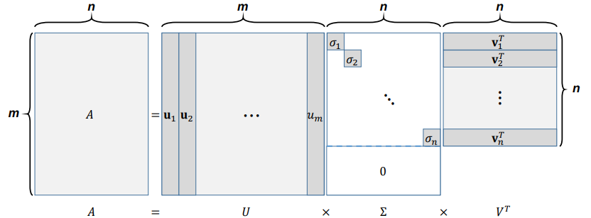
singular value decomposition (SVD) : is a factorization of a real or complex matrix that generalizes the eigendecomposition (EVD) of a square normal matrix to any $m \times n$ matrix via an extension of the polar decomposition.
$$ A = U \Sigma V^T$$ - $A \in \mathbb{R}^{m \times n}$ : A given rectangular matrix
- $U \in \mathbb{R}^{m\times m} $ : matrices with orthonormal columns, providing an orthonormal basis of $Col(A)$
- $V \in \mathbb{R}^{n \times n}$ : matrices with orthonormal columns, providing an orthonormal basis of $Row(A)$
- $\Sigma \in \mathbb{R}^{m \times n}$ : a diagonal matrix whose entries are in a decreasing order, i.e., $\sigma_1 \geq \sigma_2 \geq … \geq \sigma_{min(m,n)}$
5.2 SVD as Sum of Outer Products
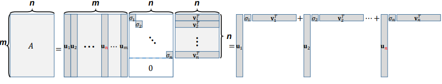
- SVD as Sum of Outer Products : $A$ can also be represented as the sum of outer products
$$ A = U \Sigma V^T = \Sigma_{i=1}^n \sigma_i \mathbf{u_j v_i^T}$$
-
From now on, we just want to show the equation below is true in this chapter (5.2) for the next chapter (5.3)
$$AV = U\Sigma \Longleftrightarrow A=U \Sigma V^T$$
-
Another Perspective of SVD : We can easily find two orthonormal basis sets, {$u_1, … , u_n$} for $Col(A)$ and {$v_1, … v_n$} for $Row (A)$, by using, Gram-Schmidt orthogonalization.
-
Are these unique orthonormal basis sets? No, then can we jointly find them such that
$$ A \mathbf{v_i} = \sigma_i \mathbf{u_i}$$
-
Let us denote $ U = \begin{bmatrix} \mathbf{u_1 \ u_2 \ … \ u_m} \end{bmatrix} \in \mathbb{R}^{m\times n}$, $ V = \begin{bmatrix} \mathbf{v_1 \ v_2 \ … \ v_n} \end{bmatrix} \in \mathbb{R}^{n \times n}$ and $ \Sigma = diag(\sigma_n) \in \mathbb{R}^{n \times n}$
-
$AV = U\Sigma \Longleftrightarrow \begin{bmatrix} A\mathbf{v_1} \ A\mathbf{v_2} \ … \ A\mathbf{v_n} \end{bmatrix} = \begin{bmatrix} \ \sigma_1 \mathbf{u_1} \ \sigma_2 \mathbf{u_2} \ … \ \sigma_n \mathbf{u_n} \end{bmatrix}$
-
$V^{-1} = V^T $ since $\mathbb{R}^{n \times n}$ has orthonormal columns.
-
Thus $AV = U\Sigma \Longleftrightarrow A=U \Sigma V^T$
5.3 Geometrical Interpretation of SVD
- Geometrical Interpretation : For every linear transformation (rectangular matrix) $A$ , one can find $n$ dimensional orthonormal basis of $V$ and transformed orthonormal basis $U$
$$A = U \Sigma V^T \Longleftrightarrow AV = U\Sigma$$
-
Furthermore : The figure below shows the orthogonal vector set $x, y$ and the linearly transformed one $Ax, Ay$.
-
And you can see two geometrical features :
- There could be one or more sets of orthogonal {$Ax, Ay$}.
- After transformed by matrix $A$, the lengths of $x,y$ are scaled by scaling factor. It is called singular value (like eigenvalue at EVD) and represented as $\sigma_1, \sigma_2, \sigma_3, …$ starting with the larger value.
5.4 Computing SVD
- First, we form $AA^T$ , $A^T A$ and then get SVD of each as followings :
$$ AA^T = U \Sigma V^T V \Sigma^T U^T = U \Sigma \Sigma^T U^T = U \Sigma^2 U^T$$
$$ A^T A = V \Sigma^T U^T U \Sigma V^T = V \Sigma^T \Sigma U^T = V \Sigma^2 V^T$$
- From the above, you can see the form of result equation is very similar to EVD:
- $U$ Is a orthogonal matrix which is from the eigen-decomposition of $AA^T$, and it is called left singular vector.
- $\Sigma$ is a diagonal matrix whose diagonal entries are equal to the square root of the eigenvalues from $AA^T$.
- $V$ is a orthogonal matrix which is from the eigen-decomposition of $A^TA$, and it is called right singular vector.
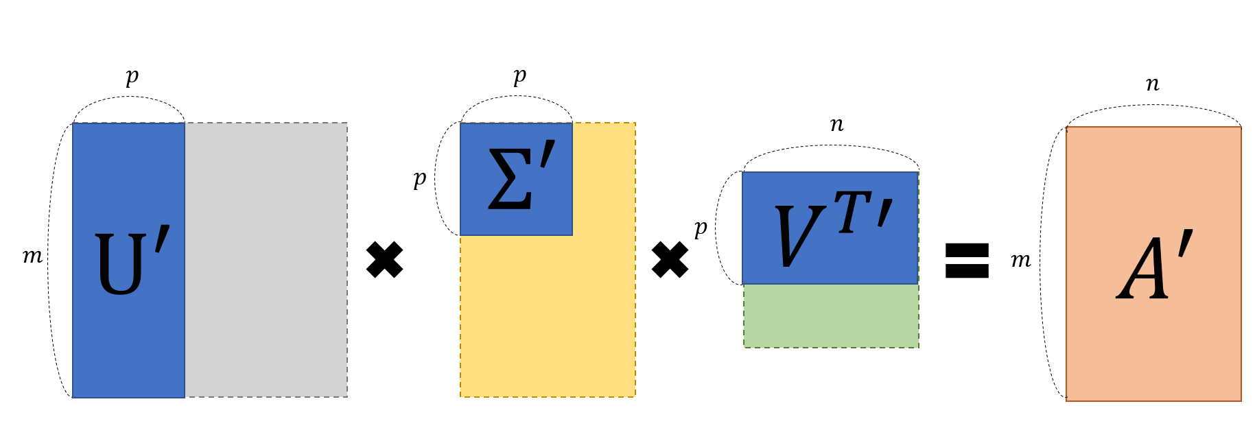
5.5 Application of SVD
- Recall SVD as Sum of Outer Products : matrix $A$ can also be represented as the sum of outer products
$$ A = U \Sigma V^T = \Sigma_{i=1}^n \sigma_i \mathbf{u_j v_i^T} = \sigma_1 \mathbf{u_1 v_1^T} + \sigma_2 \mathbf{u_2 v_2^T} + \sigma_3 \mathbf{u_3 v_3^T} …$$
-
Here, $\mathbf{u_j v_i^T} $ is $m \times n$ matrix and we can see matrix $A$ as a sum of multiple layers via SVD.
-
That is, we can reconstruct $A$ with only a few singular values rather than using all of them ($\Sigma$).
-
And this can be used for dimensionality reduction like task such as image compression.