
4.0 Introduction
-
Goal : We want to get a diagonalized matrix $D$ of a given matrix $A$ in the form of $ D = V^{-1}AV$ for some reasons such as computation resource.
-
The above diagonalization process is also called eigendecomposition ($A = VDV^{-1}$) because we can find the followings from above equation, $VD=AV$
-
$D$ is a diagonal matrix with eigenvalues in diagonal entries
-
$V$ is a matrix whose column vectors are eigenvectors
-
$A$ is a given square matrix $A \in \mathbb{R}^{n \times n}$
-
-
Consider the linear transformation $T(\mathbf{x}) = A \mathbf{x} = VDV^{-1} \mathbf{x} $, it can be seen to be a series of following transformation. (4.5.1+ 4.5.2 + 4.5.3)
-
Change of Basis
-
Element-wise Scaling
-
Back to Original Basis
-
4.1 Eigenvectors and Eigenvalues
-
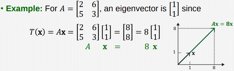
An eigenvector of a square matrix $A \in \mathbb{R}^{n \times n}$ is a nonzero vector $\mathbf{x} \in \mathbb{R}^n$ such that $A \mathbf{x} = \lambda \mathbf{x}$ for some scalar $\lambda$. In this case $\mathbf{\lambda}$ is called an eigenvalue of $A$, and such an $\mathbf{x}$ is called an eigenvector.
-
$A \mathbf{x}$ can be considered as a linear transformation $T( \mathbf{x})$. If $\mathbf{x} $ is an eigenvector, then $T(x) = A \mathbf{x} = \lambda \mathbf{x} $, which means the output vector has the same direction as $\mathbf{x}$, but the length is scaled by a factor of $\lambda$
-
And here, $8 \begin{bmatrix} 1 \\ 1 \end{bmatrix} $ is faster than $ \begin{bmatrix} 2\ 6 \\ 5 \ 3 \end{bmatrix}\begin{bmatrix} 1\ 1 \end{bmatrix} $
-
The equation $A \mathbf{x} = \lambda \mathbf{x}$ can be re-written as $$(A-\lambda I)\mathbf{x}=\mathbf{0} $$
-
$\lambda$ is an eigenvalue of an $n \times n$ matrix $A$ if and only if this equation has a nontrivial solution. (since $\mathbf{x}$ should be a nonzero vector).
-
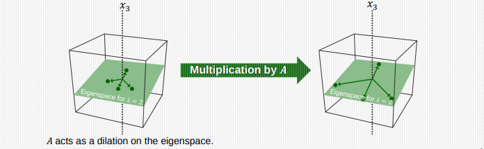
The set of all solutions of the above equation is the null space of the matrix $A-\lambda I$, which we call the eigenspace of A corresponding to $\lambda$
-
The eigenspace consists of the zero vector and all the eigenvectors corresponding to $\lambda$, satisfying the above equation.
4.2 Null Space
- Null Space : The null space of a matrix $A \in \mathbb{R}^{m\times n}$ is the set of all solutions of a homogeneous linear system, $A \mathbf{x = 0}$
- For $A = \begin{bmatrix} \mathbf{a_1^T} \\ … \\ \mathbf{a_m^T} \end{bmatrix}$, $\mathbf{x}$ should satify the following $ \mathbf{ a_1^Tx =a_2^Tx= … =a_m^Tx }=0$, That is, $\mathbf{x} $ should be orthogonal to every row vector in $A$
- Orthogonal Complement : The set of all vectors $\mathbf{z}$ that are orthogonal to $W$ is called the orthogonal complement of $W$ and is denoted by $W ^ \perp$.
4.3 Characteristic equation
$$(A - \lambda I) \mathbf{x = 0}$$
-
The set of all solutions of the above equation = null space of the matrix $(A - \lambda I)$ = eigenspace of $A$ corresponding to $\lambda$
-
The eigensapce consists of the zero vector and all the engienvectors corresponding to $\lambda$
-
How can we find the eigenvalues?
-
If $(A-\lambda I)\mathbf{x = 0}$ has a nontrivial solution, then the columns of $(A - \lambda I)$ should be noninvertible.
-
If it is invertible, $\mathbf{x}$ cannot be a nonzero vector since
$$ (A - \lambda I)^{-1} (A - \lambda I) \mathbf{x} = (A - \lambda I)^{-1} \mathbf{0} \longrightarrow \mathbf{x = 0} $$
- Thus, we can obtain eignevalues by solving characteristic equation :
$$ det(A - \lambda I) = 0$$
-
Also, the solution is not unique, and thus $A-\lambda I$ has linearly dependent columns.
-
Once obtaining eigenvalues, we compute the eigenvectors for each $\lambda$ by solving : $$ (A-\lambda I) \mathbf{x = 0}$$
-
Eigenspace : Note that the dimension of the eigenspace (corresponding to a particular $\lambda$) can be more than one. In this case, any vector in the eigenspace satisfies
$$ T\mathbf{(x)} = A \mathbf{(x)} = \lambda \mathbf{(x)}$$
-
In summary, we can find all the possible eigenvalues and eignevectors, as follows.
-
First, find all the eigenvalue by solving the characteristic equation : $ det(A-\lambda I) = 0$
-
Second, for each eigenvalue $\lambda$, solve for $(A-\lambda I) \mathbf{x=0}$ and obtain the set of basis vectors of the corresponding eigenspace.
4.4 Diagonalization
-
Diagonal matrix : matrix in which the entries outside the main diagonal are all zero
-
Diagonalization : We want to change a given square matrix $A \in \mathbb{R}^{n\times n}$ into a diagonal matrix via the following form : $D = V^{-1} A V $
-
For $A$ to be diagonalizable, an invertible $V$ should exist such that $V^{-1}AV$
-
How can we find an invertible $V$ and the resulting diagonal matrix $D$
-
$V = [\mathbf{v_1, v_2 , … , v_n}]$ where $\mathbb{v_i}$ are column vectors of $V$
-
$D = diag[\lambda_1, \lambda_2 , … , \lambda_n ]$
$$ D = V^{-1}AV $$
$$ VD = AV$$
$$AV = A[ \mathbf{v_1, v_2 , … v_n }] = [A\mathbf{v_1}, A\mathbf{v_2},…, A\mathbf{v_n}], (\text{column vector matmul})$$
$$VD = [\lambda \mathbf{v_1},\lambda \mathbf{v_2}, … ,\lambda \mathbf{v_n}]$$
$$AV=VD \longleftrightarrow [A\mathbf{v_1}, A\mathbf{v_2},…, A\mathbf{v_n}] = [\lambda \mathbf{v_1},\lambda \mathbf{v_2}, … ,\lambda \mathbf{v_n}]$$
-
From above, we obtain
$$A \mathbf{v_1} = \lambda \mathbf{v_1}, A \mathbf{v_2} = \lambda \mathbf{v_2}, … , A \mathbf{v_n} = \lambda \mathbf{v_n}$$
-
Thus $\mathbf{v_1, v_2, … v_n} $ should be eigenvectors and $\lambda_1, \lambda_2, …. \lambda_n$ should be eigenvalues.
-
Then, For $VD = AV \longrightarrow D = V^{-1}AV$ to be true, $V$ should invertible.
-
In this case, the resulting diagonal matrix D has eigenvalues as diagonal entries
- Diagonalizable matrix : For $V$ to be invertible, $V$ should be a square matrix in $\mathbb{R}^{n \times n}$, and $V$ should have $n$ linearly independent columns : Hence, $A$ should have $n$ linearly independent eigenvectors.
4.5 Eigen-Decomposition and Linear Transfomation
-
Eigendecomposition : If $A$ is diagonalizable, we can write $A = V^{-1}DV$, and we can also write $A = VDV^{-1}$, which we call eigendecomposition of $A$. So, $A$ being diagonalizable is equilvalent to $A$ having Eigendecomposition.
-
Suppose $A$ is diagonalizable, thus having eigendecomposition $ A = VDV^{-1}$, Consider the linear transformation $T(\mathbf{x}) = A \mathbf{x}$, it can be seen to be a series of following transformation. (4.5.1+ 4.5.2 + 4.5.3)
$$T(\mathbf{x}) = A\mathbf{x} = VDV^{-1}\mathbf{x} = V(D(V^{-1}\mathbf{x}))$$
4.5.1 Change of Basis
- Let $\mathbf{y} = V^{-1}\mathbf{x}$ then $V \mathbf{y=x}$
- $\mathbf{y}$ is a new coordinate of $\mathbf{x}$ with respect to a new basis of eigenvectors {$\mathbf{v_1, v_2}$}
- https://angeloyeo.github.io/2020/12/07/change_of_basis.html
4.5.2 Element-wise and Dimension-Wise Scaling
-
$T(\mathbf{x}) = V(D(V^{-1}\mathbf{x})) = V(D\mathbf{y})$
-
Let $ z=D\mathbf{y}$. This computation is a simple Element-wise scaling of $\mathbf{y}$
4.5.3 Back to Original Basis
-
$T(\mathbf{x}) = V(D\mathbf{y}) = Vz$
-
$z$ is still a coordinate based on the new basis $\mathbf{v_1, v_2}$
-
$Vz$ converts $z$ to another coordinates based on the original standard basis.
-
That is, $Vz$ is a linear combination of $\mathbf{v_1}$ and $\mathbf{v2}$ using the coefficient vector $z$.
-
That is,
$$Vz = \begin{bmatrix} \mathbf{v_1} \ \mathbf{v_2} \end{bmatrix} \begin{bmatrix} z_1 \ z_2 \end{bmatrix} = \mathbf{v_1}z_1 + \mathbf{v_2}z_2$$
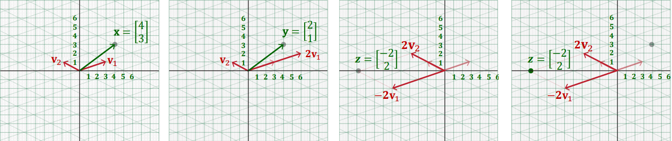
Example : $A = VDV^{-1} = \begin{bmatrix} 3&{-2}\\ 1&1 \end{bmatrix} \begin{bmatrix} -1&0\\ 0&2 \end{bmatrix}\begin{bmatrix} 3&{-2}\\ 1&1 \end{bmatrix}^{-1}, \text{ and } \bf{x}=\begin{bmatrix} 4\\ 3 \end{bmatrix} $
$$ y = \begin{bmatrix} 3&{-2}\\ 1&1 \end{bmatrix}^{-1}\begin{bmatrix} 4\\ 3 \end{bmatrix} = \begin{bmatrix} 2\\ 1 \end{bmatrix} $$
$$ z = \begin{bmatrix} -1 & 0\\ 0 &2 \end{bmatrix} \begin{bmatrix} 2\\ 1 \end{bmatrix} = \begin{bmatrix} -2\\ 2 \end{bmatrix}$$
$$ Vz = \begin{bmatrix} 3&{-2}\\ 1&1 \end{bmatrix}\begin{bmatrix} -2\\ 2 \end{bmatrix} = \begin{bmatrix} -10\\ 0 \end{bmatrix} $$
4.5.4 Linaer Transformation via $A^k$
-
Now, consider recursive transformation $A \times A \times A … \times A \mathbf{x} = A^k \mathbf{x} $
-
If $A$ is diagonalizable, $A$ has Eigendecomposition
$$ A = VDV^{-1}$$
$$ A^k = (VDV^{-1})(VDV^{-1})(VDV^{-1})…(VDV^{-1}) = (VD{^k}V^{-1})$$
-
Here, $D^k$ is simply computed as $diag[\lambda_1^k, \lambda_2^k… , \lambda_n^k]$
-
It is much faster to compute $V(D^k(V^{-1}\mathbf{x}))$ than to compute $A^k \mathbf{x}$
Summary
-
Eigenvalue and Eigenvectors
-
Null space, Column space, and orthogonal complement in $\mathbb{R}^n$
-
Diagonalization and Eigendecomposition
-
Linear transforamtion via eigendecomposition