Linear Algebra for ML #3 | Least Square

2019-07-01 1. Linear Algebra Comments

3.0 Least Square

Inner Product : Given $ \mathbf{u,v} \in \mathbb{R}^n$, we can consider $ \mathbf{u,v} $ as $n \times 1$ matrices. The number $\mathbf{u^Tv}$ is called inner product or dot product, and it is written as $ \mathbf{u \cdot v} $.
Vector Norm : The length or magnitude of $\mathbf{v}$, can be calculated as $ \sqrt{ \mathbf{v} \cdot \mathbf{v} }$
$L_p$ Norm : $ \Vert \mathbf{x} \Vert_p = ( \Sigma_{i=1}^n \vert x_i \vert^p)^{1/p}$
Euclidean Norm : $L_2$ norm
Frobenius Norm : can be seen as an expansion of $L_2$ norm to apply to the matrix : $ \Vert A \Vert_F = \sqrt{\Sigma_{i=1}^m \Sigma_{j=1}^n} \vert a_{ij}\vert^2$
Unit Vector : A vector whose length is 1
Normalizing : Given a nonzero vector $\mathbf{v}$, if we divide it by its length, we obtain a unit vector.
Distance between vectors : dist($\mathbf{u,v}$) = norm($\mathbf{u-v}$) = $\Vert \mathbf{u-v} \Vert$
Inner Product and Angle Between Vectors : $\mathbf{u \cdot v} = \mathbf{\Vert u \Vert \Vert v \Vert} cos \theta $
Orthogonal Vectors : $\mathbf{u \cdot v} = \mathbf{\Vert u \Vert \Vert v \Vert} cos \theta = 0$. That is $ (\mathbf{u \perp v})$

3.1 Introduction to Least Squares Problem

Over-Determined : number of equations > number of variables (we have much more data examples), usually no solution exists
Motivation for Least Squares : Even if no solution exists, we want to approximately obtain the solution for an over-determined system.

The example below shows how to determine which solution is better between $\begin{bmatrix} -0.12 \\ 16 \\ -9.5 \end{bmatrix}$ and $\begin{bmatrix} -0.4 \\ 20 \\ -20 \end{bmatrix}$ for given Over-Determined System.

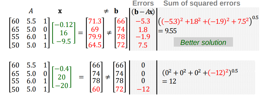
Least Squares Problem : Given an over-determined system, $A \mathbf{x \simeq b}$, a least squares solution $\hat{x}$ is defined as

$$\mathbf{\hat{x}} = argmin_x | \mathbf{b} - A \mathbf{x} | $$

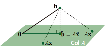
The most important aspect of the least-squares problem is that no matter what $\mathbf{x}$ we select, the vector $A \mathbf{x}$ will necessarily be in the column space Col $A$
Thus, we seek for $\mathbf{x}$ that makes $A \mathbf{x}$ as the closest point in Col $A$ to $\mathbf{b}$

3.2 Geometric Interpretation of Least squares

Consider $ \mathbf{\hat{x}} $ such that $ \hat{b} = A\mathbf{\hat{x}} $ is the closest point to $\mathbf{b}$ among all points in Column Space of $A$.
That is, $\mathbf{b}$ is closer to $\mathbf{\hat{b}}$ than to $A \mathbf{x}$ for any other $\mathbf{x}$.
To satisfy this, the vector $\mathbf{b}- A\mathbf{\hat{x}}$ should be orthogonal to Col $A$
This means $\mathbf{b} - A \mathbf{\hat{x}}$ should be orthogonal to any vector in Col A:

$$ \mathbf{b} - A\mathbf{\hat{x}} \perp (x_1\mathbf{a}_1 + …. x_p\mathbf{a}_n)$$

Or equivalently,

$$ A^T(\mathbf{b} - A\hat{\mathbf{x}}) = 0$$

$\mathbf{b} - A \mathbf{\hat{x}} \perp \mathbf{a_1} \rightarrow >\mathbf{a}_1^T(\mathbf{b} - A \mathbf{\hat{x}})=0 $
$\mathbf{b} - A \mathbf{\hat{x}} \perp \mathbf{a_2} \rightarrow >\mathbf{a}_2^T(\mathbf{b} - A \mathbf{\hat{x}})=0 $ …
$\mathbf{b} - A \mathbf{\hat{x}} \perp \mathbf{a_m} \rightarrow >\mathbf{a}_m^T(\mathbf{b} - A \mathbf{\hat{x}})=0 $

same with the equation below which is called a normal equation

$$A^T A\hat{\mathbf{x}}= A^T\mathbf{b}$$

3.3 Normal Equation

given a least squares problem, $Ax \simeq \mathbf{b}$ , we obtain normal equation

$$A^T A\hat{\mathbf{x}}= A^T\mathbf{b}$$

if $A^T A$ is invertible, then the solution is computed as

$$\hat{\mathbf{x}}= (A^T A)^{-1} A^T\mathbf{b} $$

If $A^T A$ is not invertible, the system has either no solution or infinitely many solutions. However, the solution always exist for this “normal” equation, and thus infinitely many solutions exist.
If and only if the columns of $A$ are linearly dependent, $A^TA $ is not invertible. However, $A^T A$ is usually invertible.

3.4 Orthogonal Projection

consider the orthogonal projection of $\mathbf{b}$ onto Col $A$ as

$$ \mathbf{\hat{b}} = f(\mathbf{b})= A{\mathbf{\hat{x}}} = A(A^TA)^{-1}A^T\mathbf{b} $$

Orthogonal set : A set of vectors {$ \mathbf{u_1, … u_p}$} in $\mathbb{R^n}$ if each pair of distinct vectors from the set is orthogonal. That is, if $\mathbf{u_i \cdot u_j}=0$ whenever $i \neq j$. So, All vectors in the orthogonal set are orthogonal to each other.
Orthonormal set : A set of vectors {$ \mathbf{u_1, … u_p}$} in $\mathbb{R^n}$ if it is an orthogonal set of unit vectors (norm=1) .
Orthogonal and Orthonormal Basis : Consider basis {$\mathbf{v_1, … , v_p}$} of a p-dimensional subspace $W $ in $\mathbb{R}^n$. We can make it as an orthogonal(or orthonormal) basis using Gram-Schmidt process.

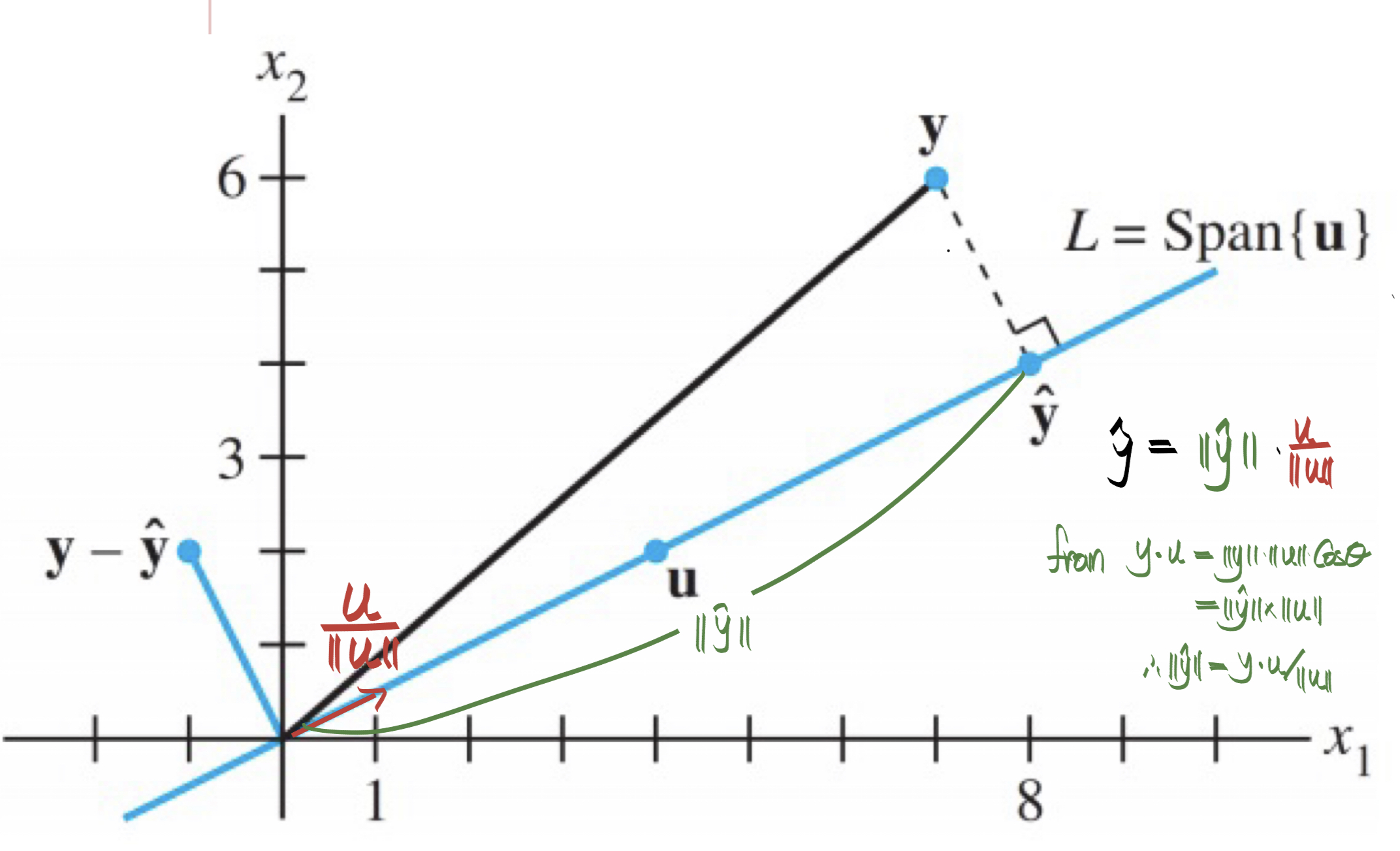
Orthogonal Projection $\hat{\mathbf{y}}$ of $\mathbf{y}$ onto Line : Consider the orthogonal projection $\hat{\mathbf{y}}$ of $\mathbf{y}$ onto Line (1D subspace $L$). From the above picture, $\hat{\mathbf{y}}$ can be represented by multiplication of the norm (length) for $\hat{\mathbf{y}}$ (=$ | | \hat{\mathbf{y}} | |$) and the unit vector of $\mathbf{u}$ ( = $\mathbf{\frac{u}{||u||}} $ ). And we can calculate $\hat{\mathbf{y}}$ from the inner product of $\mathbf{y} \text{ and } \mathbf{u}$

$$ \hat{\mathbf{y}} = proj_L(\mathbf{y})$$

$$ = | | \hat{\mathbf{y}} | | \cdot \mathbf{\frac{u}{||u||}} = \mathbf{\frac{y \cdot u}{||u||}} \cdot \mathbf{\frac{u}{||u||}} $$

$$= \mathbf{\frac{y \cdot u}{u \cdot u}} \cdot \mathbf{u}, ( \because \mathbf{||u||}^2 = \mathbf{u \cdot u})$$

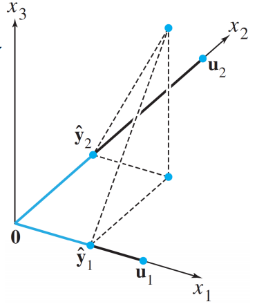
Orthogonal Projection $\hat{\mathbf{y}}$ of $\mathbf{y}$ onto Plane : Consider the orthogonal projection $\hat{\mathbf{y}}$ of $\mathbf{y}$ onto two-dimensional subspace $W$

$$ W = span ( \mathbf{u_1, u_2} ) $$

$$ \hat{\mathbf{y}} = proj_L(\mathbf{y}) = \mathbf{\frac{y \cdot u_1}{u_1 \cdot u_1}} \cdot \mathbf{u_1} +\mathbf{\frac{y \cdot u_2}{u_2 \cdot u_2}} \cdot \mathbf{u_2} $$

Orthogonal Projection as a Linear Transformation : Consider a transformation of orthogonal projection $\mathbf{\hat{b}}$ of $\mathbf{b}$. If orthonormal basis {$\mathbf{u_1, u_2}$} of a subspace $W$ is given, both $\mathbf{u_1, u_2}$ are unit vector and we can get following equation :

$$ \mathbf{\hat{b}} = f(\mathbf{b}) = \mathbf{ (b \cdot u_1)u_1 + (b \cdot u_2 )u_2 } $$

$$ \mathbf{ = (u_1^Tb)u_1 + (u_2^T b)u_2 = (u_1u_1^T + u_2 u_2^T)b = \begin{bmatrix} u_1^T \\ u_2^T \end{bmatrix} \begin{bmatrix} u_1 \ u_2 \end{bmatrix} = UU^T b } $$

3.5 Gram-Schmidt Orthonomalization

If two (or more) vectors are linearly independent, these vectors create an vector space. And we want to represent this vector space using a orthogonal (or orthonormal) set in many cases.
In the previous chapter, we’ve learned orthogonal projection of one vector to the other.
From this we can represent a given vector space (linearly independent vector set) with a orthogonal vector set : Gram-Schmidt

Example: Let $W=span( \mathbf{x_1, x_2})$, where $\mathbf{x_1} = \begin{bmatrix} 3\\ 6\\ 0\end{bmatrix}$, $\mathbf{x_2} = \begin{bmatrix} 1\\ 2\\ 2\end{bmatrix}$. Construct an orthogonal basis {$\mathbf{v_1, v_2}$} for $W$

Solution:

Let $\mathbf{v_1} = \mathbf{x_1}$. And, let $\mathbf{v_2}$ the component of $\mathbf{x_2}$ is orthogonal to $\mathbf{x_1}$, i.e. $$ \mathbf{v_2 = x_2 - proj_{v1}(x2) = x_2 - \frac{x_2 \cdot x_1}{x_1 \cdot x_1} x_1 }= \begin{bmatrix} 1 \\ 2 \\ 2 \end{bmatrix} - \frac{15}{45}\begin{bmatrix} 3 \\ 6 \\ 0 \end{bmatrix} = \begin{bmatrix} 0 \\ 0 \\ 2 \end{bmatrix} $$

Now, we get orthogonal basis for $W$. That is, $$\mathbf{v_1} = \begin{bmatrix} 3\\ 6\\ 0\end{bmatrix}, \mathbf{v_2} = \begin{bmatrix} 0\\ 0\\ 2\end{bmatrix}$$

We can get the orthonormal set $\mathbf{(u_1,u_2)}$ of these vectors by dividing the norm of each vectors $$\mathbf{u_1} = \frac{1}{\sqrt{45}} \begin{bmatrix} 3\\ 6\\ 0\end{bmatrix}, \mathbf{u_2} = \begin{bmatrix} 0\\ 0\\ 1 \end{bmatrix}$$

3.6 QR Factorization (QR Decomposition)

QR Decomposition : is a decomposition of a matrix $A$ into a orthogonal matrix $Q$ (with Gram-Schmidt) and upper triangular matrix $R$ .
1. For a given lineary independent matrix, we can find orthogonal basis of the vector space using Gram-Schumidt.
2. There should be another matrix that undo the above orthogonalization tranfrom
3. Here, the orthogonalized matrix is represented as $Q$ and the ‘un-doing’ matrix is represented as $R$.

$$A \rightarrow \text{Gram-Schumidt} \rightarrow Q \rightarrow \times R \rightarrow A $$

Example : Consider the decomposition of linearly independeny matrix $A = \begin{bmatrix} 12&-51&4\\ 6&167 &-68\\ -4&24&-41\end{bmatrix}$

Solution :

Then, we can calculate $Q$ by means of Gram-Schmidt as follows:

$$U = [\mathbf{u1, u2, u3}] = \begin{bmatrix} 12&-69&-58/5\\ 6&158 &-6/5\\ -4&30&-33\end{bmatrix}$$

$$ Q = [\mathbf{\frac{u_1}{|u_1|}, \frac{u_2}{|u_2|}, \frac{u_3}{|u_3|}}] = \begin{bmatrix} 6/7&-69/175&-58/175\\ 3/7&158/175 &-6/175\\ -2/7&30/175&-33/35\end{bmatrix} $$

Thus, we have

$$R = Q^TA = \begin{bmatrix} 14&21&-14\\ 0&175 &-70\\ 0&0&35\end{bmatrix}$$

Summary

Least Square Problem : No solution exists for the linear equation $Ax=b$

=> Approximate the solution $\hat{x}$ minimizes $ b - A \hat{x}$.

=> And $ b - A \hat{x}$ should be orthogonal to Column Space => $ A^T(\mathbf{b} - A\hat{\mathbf{x}}) = 0$

=> From this equation, We get the normal equation $A^T A\hat{\mathbf{x}}= A^T\mathbf{b}$

=> And if $A^T A$ is invertible, the solution $\hat{\mathbf{x}}= (A^T A)^{-1}A^T\mathbf{b}$

=> On the other view, $\hat{b}$ is the orthogonal projection of $b$

=> Now, we can find orthogonal projection of a vector

=> we can find orthogonal vector set using given linearly independ vectors (in that vector space)