
2.1 Linear Equation and Linear System
- Linear Equation is an equation that can be written in the form $$ a_1x_1 + …. a_nx_n = b $$
- The above equation can be written as $ \textbf{a}^T \textbf{x} = b $.
- Linear System is a collection of one or more linear equations
-
Identity Matrix : $I$ is a square matrix whose diagonal entries are all 1’s and all the other entries are zeros.
-
Inverse Matrix : $A^{-1}$ is defined such that $A^{-1}A = AA^{-1} = I$
$$A^{-1} = \frac{1}{ad-bc} \begin{bmatrix} d&{-b}\\ -c&a \end{bmatrix}$$
-
Determinant : $det(A) = ad-bc$ determines whether $A$ is invertible
-
If $A$ is non invertible, $A \textbf{x} = \textbf{b}$ will have either no solution or infinitely many solutions.
2.2 Linear Combination
-
For given vectors $\textbf{v}_1,\textbf{v}_2, … \textbf{v}_p $ and given scalars $ c_1, c_2, … c_p $,
$ c_1\textbf{v}_1 + c_2 \textbf{v}_2, … + c_p \textbf{v}_p $ is called Linear Combination of vectors with weights $c$.
- Span : Span{$\textbf{v}_1, … \textbf{v}_p$} is defined as the set of all linear combinations of $\textbf{v}_1, … \textbf{v}_p$. That is, Span is the collection of all vectors that can be written in the form $ c_1\textbf{v}_1 + c_2 \textbf{v}_2, … + c_p \textbf{v}_p $.
- Geometric Description of Span : $ \textbf{v}_1 $ and $\textbf{v}_2$ are in $\mathbb{R}^3$ then Span is the plane in $\mathbb{R}^3$ that contains $ \textbf{v}_1 $ and $\textbf{v}_2$
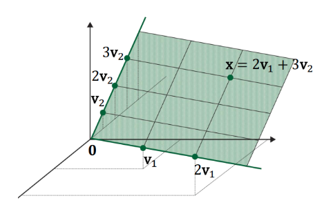
- Geometric Interpretation of Vector Equation : we can find whether the solution of vector equation exists using the knowledge of span. The solution of below vector equation exists only when $ \textbf{b} \in Span(\textbf{a}_1, \textbf{a}_2, \textbf{a}_3) $.
$$\textbf{a}_1 x_1 + \textbf{a}_2 x_2 + \textbf{a}_3 x_3 = b $$
- Matrix Multiplications as Linear Combinations of Vectors :
$$ \begin{bmatrix} 60&1.7&1 \\ 65&1.6&0 \\ 55&1.8&1 \end{bmatrix} \begin{bmatrix} x_1 \\ x_2 \\ x_3 \end{bmatrix} = \begin{bmatrix} 60\\ 65\\ 55\end{bmatrix} x_1 + \begin{bmatrix} 1.2 \\ 1.6 \\ 1.8 \end{bmatrix} x_2 + \begin{bmatrix} 1 \\ 0 \\ 1 \end{bmatrix} x_3 $$
- Matrix Multiplication as Column Combinations
$$ \begin{bmatrix} 1&1&0 \\ 1&0&1 \\ 1&-1&1 \end{bmatrix} \begin{bmatrix} 1 \\ 2 \\ 3 \end{bmatrix} = \begin{bmatrix} 1\\ 1\\ 1\end{bmatrix}1 + \begin{bmatrix} 1\\ 0\\ -1\end{bmatrix}2 + \begin{bmatrix} 0\\ 1\\ 1\end{bmatrix}3 $$
- Matrix Multiplication as Row Combinations
$$ \begin{bmatrix} 1&2&3 \end{bmatrix} \begin{bmatrix} 1&1&0 \\ 1&0&1 \\ 1&-1&1 \end{bmatrix} = 1 \times \begin{bmatrix} 1&1&0 \end{bmatrix} + 2\times \begin{bmatrix} 1& 0&1 \end{bmatrix} + 3 \times \begin{bmatrix} 1& -1& 1\end{bmatrix}$$
- Matrix Multiplication as Sum of Outer Products
$$\begin{bmatrix} 1&1 \\ 1&-1 \\ 1&1 \end{bmatrix} \begin{bmatrix} 1& 2& 3 \\ 4&5&6 \end{bmatrix} = \begin{bmatrix} 1\\ 1\\ 1\end{bmatrix} \begin{bmatrix} 1& 2& 3\end{bmatrix} + \begin{bmatrix} 1\\ -1\\ 1\end{bmatrix} \begin{bmatrix} 4& 5& 6\end{bmatrix} $$
2.3 Linear Independence
-
The solution for $A \textbf{x} = \textbf{b} $ is unique, when $\textbf{a}_1, \textbf{a}_2, \textbf{a}_3 $ are linearly independent
-
Infinitely many solutions exists when $\textbf{a}_1, \textbf{a}_2, \textbf{a}_3 $ are linearly dependent.
- Linear Independence (practical) : Given a set of vectors $ \textbf {v}_1 , … , \textbf {v}_p $ , check if $ \textbf{v}_j$ can be represented as a linear combination of the previous vectors. If at least one such $ \textbf{v}_j$ is found then $ \textbf {v}_1 , … , \textbf {v}_p $ is linearly dependent.
- Linear Independence (Formal) : Consider $ x_1 \textbf{v}_1 + … + x_p \textbf{v}_p = \textbf{0} $. Obviously, one solution is $\textbf{x} = [0…0]$, which we call a trivial solution. If this is the only solution $ \textbf {v}_1 , … , \textbf {v}_p $ is the only solution. if this system also has other nontrivial solutions, $ \textbf {v}_1 , … , \textbf {v}_p $ are linearly dependent.
2.4 Basis of a Subspace
-
Subspace : is defined as a subset of $\mathbb{R}^n$ closed under linear combination
-
A subspace is always represented as Span {$\mathbf{v}_1 , … , \mathbf{v}_p$}
- Basis of a subspace : a set of vectors that satisfies both of the following
-
Fully spans the given subspace $H$
- Linearly independent (i.e., no redundancy)
- Non-Uniqueness of Basis : In the subspace $H$ (green plane), there other set of linearly independent vectors that span the subspace $H$
- Dimension of Subspace : Even though different basis exist for $H$, the number of vectors in any basis for $H$ will be unique. This number is the dimension of $H$.
- Column Space of Matrix : the subspace could be spanned by the column vector of $A$.
- Rank of Matrix : the dimension of the column space of $A$
Details
$$ A = \begin{bmatrix} 1&0&2 \\ 0&1&1 \\ 1&0&2 \end{bmatrix}, \ \ \text{ Column Vector } a_1, a_2, a_3 = \begin{bmatrix} 1\\ 0\\ 1\end{bmatrix} , \begin{bmatrix} 0\\ 1\\ 0\end{bmatrix}, \begin{bmatrix} 2\\ 1\\ 2\end{bmatrix} $$
-
Column Space is subspace of column vectors from matrix $A$. And we need to find basis vector to get column space.
-
$a_1, a_2$ is independent each other. $a_3$ is represented as linear combination of $a_1, a_2$ . As a result, $a_3$ is dependent on $a_1, a_2$. So, $a_1, a_2$ become basis vector for colum space of $A$
-
Here, Rank of matrix $A$ is two. Because we have only two vectors $a_1, a_2$ that are linearly independent.
-
If a solution for $A \textbf{x} = \textbf{b} $ exists, then $b$ must be on the column space of $A$. Because, $b$ is linear combination of column vectors
$$ Ax = \begin{bmatrix} 1&0&2 \\ 0&1&1 \\ 1&0&2 \end{bmatrix} \begin{bmatrix} x_1\\ x_2\\ x_3\end{bmatrix} = \begin{bmatrix} 1\\ 0\\ 1\end{bmatrix} x_1 + \begin{bmatrix} 0\\ 1\\ 0\end{bmatrix} x_2 + \begin{bmatrix} 2\\ 1\\ 2\end{bmatrix} z_3 = \begin{bmatrix} b_1\\ b_2\\ b_3\end{bmatrix} $$
2.5 Chage of Basis
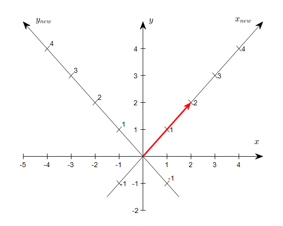
- Generally, vectors are defined on cartesian coordinate , and it means they are based on standard basis (1,0), (0,1).
- But sometimes, we need vectors on different coordinate (basis) for some reasons like computational efficiency. (e.g. eigendecomposition)
- When the coordinate changes, the vector itself does not changed, but the representation of vector has been changed from (2,2) to (2,0) as in figure below
2.6 Linear Transformation
-
A transformation, function, or mapping maps an input $x$ to an output $y$
-
Domain : Set of all the possible values of $x$
-
Co-Domain : Set of all the possible values of $y$
-
Range : Set of all the output values mapped by each $x$ in the domain
-
Linear Transforamtion : A transformation (or mapping) $T$ is linear if : $$ T(c \mathbf{u}+ d \mathbf{v}) = cT (\mathbf{u}) + dT(\mathbf{v})$$
-
Matrix of Linear Transformation : In general, let $T$ : $ \mathbb{R}^n \rightarrow \mathbb{R}^m $ be a linear transformation. Then $T$ is always written as a matrix-vector multiplication. i.e., $T(\mathbf{x}) = A \mathbf{x}$
-
Here, the matrix $A$ is called the standad matrix of the linear transformation.
2.7 Linear Transformation in Neural Networks
-
Fully Connected Layers can be thought as a linear transformation
-
Fully Connected Layers usually involve a bias term, That’s why we call it an affine layer, not a linear Layers
-
Reference : colah’s blog
2.8 ONTO and ONE-TO-ONE
-
ONTO : A mapping $T$ : $\mathbb{R}^n \rightarrow \mathbb{R}^m$ is said to be onto $\mathbb{R}^m$ if each $\mathbf{b} \in \mathbb{R}^m$ is the image of at least one $x \in \mathbb{R}^n$. That is, the range is equal to the co-domain.
-
ONE-TO-ONE : A mapping $T$ : $\mathbb{R}^n \rightarrow \mathbb{R}^m$ is said to be one-to-one if each $\mathbf{b} \in \mathbb{R}^m$ is the image of at most one $x \in \mathbb{R}^n$. That is, each output vector in the range is mapped by only one input vector, no more than that.